Explicit Credit Assignment through Local Rewards and Dependence Graphs in Multi-Agent Reinforcement Learning

Bang Giang Le; Viet Cuong Ta

REVIEW 4 major objections 4 minor 3 references

Explicit Credit Assignment through Local Rewards and Dependence Graphs in Multi-Agent Reinforcement Learning

T0 review · 4 major / 4 minor · reviewed 2026-08-03 · deepseek-v4-flash

Challenge this review Re-run · record.json Download PDF Read on arXiv ↗ Review JSON

Pith's one-line read The paper proves that in cooperative multi-agent reinforcement learning, cross-agent policy-gradient terms before the first causal path in a dependence graph are exactly zero, making truncation exact rather than approximate.

desk verdict A genuinely novel policy-gradient truncation result on dependence graphs that deserves a serious look, though the practical estimator does not inherit the exactness of the theory. read the letter →

arxiv 2601.21523 v2 pith:Y6TZH5KS submitted 2026-01-29 cs.LG

Bang Giang Le , Viet Cuong Ta This is my paper · ORCID

classification cs.LG

keywords multi-agentreinforcementlearningcreditassignmentpolicygradientdependencegraphnetworkedMDPlocalrewardsgeneralizedadvantageestimationreverseworldmodel

verification ladder T0 review T1 audit T2 compute T3 formal

The pith

A machine-rendered reading of the paper's core claim, the machinery that carries it, and where it could break.

The reading

Cooperative multi-agent reinforcement learning usually forces a choice: give every agent the same global reward and struggle to assign credit, or give each agent its own local reward and risk selfish, myopic behavior. This paper tries to combine both by using a state dependence graph that tracks which agents can actually influence which other agents over time. The central claim is that an agent's policy gradient with respect to another agent's return only needs reward terms that arrive after the first timestep at which a causal path exists between them in the graph; before that, the cross-agent gradient is exactly zero. Truncating those terms is therefore not an approximation, and it removes the variance that global reward scalarization injects. The paper also gives a practical way to learn the graph from data and shows empirically that the approach beats both extreme reward settings on cooperative benchmarks.

What carries the argument

The central object is the state dependence graph of a networked MDP: a directed graph whose vertices are (state, agent) pairs and whose edges record which agents' states and actions can affect which other agents' next substates. The theorem that carries the argument is the k-hop-parent expansion: the set of agents that can have influenced agent i by time t grows monotonically, so the first meeting timestep t′ partitions the reward stream into zero and nonzero contributions. The practical machinery is a reverse world model that predicts one agent's action from another agent's state and next state; the entropy drop produced by conditioning on the second agent is thresholded to add an edge, and

What would settle it

Construct a minimal two-agent MDP where one agent's next state depends on another agent's action only when an external flag flips at the same time, so that the influencing agent is in the true parent set only intermittently and cannot be inferred from the affected agent's substate alone; then compare the exact cross-agent gradient to the paper's estimator. A nonzero difference before the estimated meeting timestep would falsify the claimed exactness for the implemented estimator.

Watch

Extended reading notes

Core claim

On the paper's own terms, the discovery is Proposition 5.1: fix any joint policy and any pair of agents i and j, and define t′ as the first timestep at which a directed path exists in the state dependence graph from (s0, j) to (s_{t′}, i). Then the policy gradient of agent j's policy with respect to agent i's cumulative return is the expectation of ∇logπ_j(a_0^j|s_0^j) times the expected discounted sum of i's rewards from t′ onward. Before t′, all cross-agent gradient contributions vanish exactly; if no such path ever exists, the cross-agent gradient is zero. The paper further shows that using an approximate graph with model error ε yields a gradient error bounded by O(B_j γ ε R_max/(1−γ)^2)

Load-bearing premise

The entire exactness result rests on the assumption that each agent's current substate is enough to identify which other agents' states and actions can influence its next substate; if that one-step locality fails, the learned graph and the meeting timesteps no longer align with true causal influence.

Editorial extensions

If this is right

If the true dependence graph is known, the dependency-graph policy gradient is unbiased and lower variance than the vanilla global-reward gradient, because it discards reward terms that cannot be causally influenced.
For sparse interaction graphs, cross-agent gradient contributions effectively vanish until the meeting timestep, so the method interpolates between local-reward learning (empty graph) and global-reward learning (fully connected graph).
When only an approximate graph is available, the error bound in Lemma 5.2 gives a principled target: learn a transition model with small total variation error ε, and the gradient bias stays O(ε/(1−γ)^2).
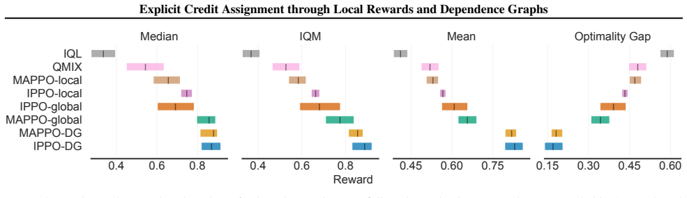
The proposed graph-estimation method makes the framework applicable when no hand-designed graph exists; empirically it performs close to an oracle graph on the tested cooperative foraging tasks.

Reading between the lines

Editorial extensions of the paper, not claims the author makes directly.

Editorial inference: the same truncation principle should transfer to off-policy and value-based learners, since the zero-gradient result is about the MDP structure rather than the policy-gradient estimator; a value-based analogue would replace reward truncation with a first-meeting value function.
Editorial inference: if the dependence graph is sparse and stable across states, the sample complexity of cooperative credit assignment could scale with the size of interaction neighborhoods rather than the total number of agents, weakening the known many-agents scalability barrier.
Editorial inference: the learned reverse-world-model graph could serve as a diagnostic for interaction structure, but the paper's own simplification (dropping state-state mutual information) suggests it will under-report edges in environments where transitions are driven by states rather than actions.
Editorial inference: the assumption that parent sets can be inferred from current substates is the main practical gap; in partially observable settings, using a recurrent policy or an observation-history encoder could recover the missing outsider influences that the one-step graph misses.

Share X Bluesky LinkedIn Reddit HN

Signed reviews

No signed human review yet.

Editorial analysis

A structured set of objections, weighed in public.

Desk editor's note, referee report, and a circularity audit.

Desk Editor's Note

read the letter

Colleague —

The paper is a serious effort, and the central idea is better than the packaging suggests. Proposition 5.1 gives a clean exact identity: for a factored networked MDP with observable parent sets, the cross-agent policy gradient is zero until the first time a path exists in the dependence graph from the acting agent to the rewarded agent. That is a neat formalization of "credit starts to flow when influence can flow," and the proof is straightforward and readable. The GAE-style aggregation over meeting times is a sensible way to make the estimate robust to noisy graphs, and the reverse-world-model edge estimator is a practical way to get the graph from data. The LBF experiments show consistent gains over both local and global reward baselines; the SMAClite numbers are honestly reported as mostly comparable.

The soft spots are real but not fatal. The biggest one is the gap between the exact theory and the implemented estimator. Proposition 5.1 is exact only for the true graph; the algorithm uses a learned graph with two explicit approximations (dropping the state mutual information, conditioning on (s_i,a_i) instead of the full parent set) and a threshold c=0.9 with no sensitivity analysis. The error lemma (Lemma 5.2) is stated for a kernel satisfying a uniform total variation bound, but the bound actually derived in inequality (4) is in expectation, so the formal guarantee does not carry over to the heuristic graph. The appendix's own limitation note says the effect of ignoring state MI is unknown and may fail when transitions depend heavily on states. None of this makes the paper incoherent—the authors admit the limitations explicitly—but it does mean the headline "exact truncation" belongs to the idealized setting, not the code.

The experiments would be stronger with confidence intervals and seed counts; Figure 4 gives aggregated metrics but no error bars. That is an addressable issue.

Who should read it: anyone working on MARL credit assignment or factored MDPs. The theory section alone is worth a look.

Verdict: worth a serious peer review. Not a desk reject. A good referee will push the authors to close the gap between the exact result and the practical estimator, and to be precise about what the experiments actually show.

Best, [Your name]

Referee Report

4 major / 4 minor

Summary. The paper proposes a dependence-graph policy gradient for cooperative MARL. Under a networked-MDP factorization in which each agent's next substate depends only on the states and actions of a state-dependent parent set, Proposition 5.1 claims that the cross-agent policy-gradient term ∇_{π^j} J^i(π) can be exactly truncated: only rewards received after the first time t' at which a path in the dependence graph connects (s_0,j) to (s_t',i) contribute. It then introduces a practical method for approximating the graph with reverse world models and a mutual-information surrogate, and a GAE-style estimator that aggregates over multiple estimated meeting times. Experiments on LBF and SMAClite with MAPPO and IPPO backbones compare the method with local-reward and global-reward baselines, and an ablation compares the learned graph with random and oracle graphs. The paper is supported by an appendix containing proofs and additional experimental detail.

Significance. If the central claims held as stated, the paper would make a useful contribution: it identifies a time-dimension truncation of policy gradients that is exact for an oracle dependence graph, complements existing spatial k-hop approximations, and is accompanied by public code and a reasonably careful evaluation protocol (IQM, ablations, multiple scenarios). The formal framework is self-contained given the networked-MDP axioms, and the authors are candid about several limitations. However, the headline exactness property is established only for a true, observable dependence graph, and the bridge from that result to the implemented approximate-graph algorithm is incomplete. In particular, the proof of Lemma 5.2 has a gap, and the practical graph estimator uses heuristics that are not covered by the lemma's assumptions. These issues are load-bearing for the paper's claimed theory, so the manuscript requires substantive revision.

major comments (4)

[Appendix A.5, proof of Lemma 5.2] The displayed equation for Q_{P,G'}^{i,j}(s,a) - Q_{P',G'}^{i,j}(s,a) is not bounded correctly. The first term contains P(s'|s,a) Q_{P,G'}(s',a') minus P'(s'|s,a) Q_{P',G'}(s',a'); after adding and subtracting P'(s'|s,a) Q_{P,G'}(s',a'), one obtains γ Σ(P-P') E Q_{P,G'} plus γ E_{P',π}[Q_{P,G'} - Q_{P',G'}]. The second of these is a recursive term that cannot be ignored. The proof bounds the first term solely by γ ε R_max/(1−γ), which yields the stated O(γ ε/(1−γ)^2) only if the recursive term is also handled. As written, the proof of the T2 bound is incomplete. A correct argument via the augmented-state simulation lemma may be possible, but it must be supplied explicitly.
[§5.2–5.3, Eq. (4) and Algorithm 2] The connection between Lemma 5.2 and the implemented graph estimator is not established. Lemma 5.2 requires a uniform sup-norm TV bound ε on the transition kernels. Inequality (4) provides only an expectation bound under some state-action distribution. Moreover, Section 5.3 introduces two further simplifications — dropping I(S_i';S_j) and replacing parent sets by (s_i,a_i) — and then applies a heuristic threshold c=0.9. No argument is given that the resulting graph G' satisfies the hypothesis of Lemma 5.2, or even a distributional analogue with explicit ε. Thus the exactness of Proposition 5.1 does not transfer to the algorithm whose results are reported; the practical method is best described as a heuristic. The authors should either weaken the theoretical claims accordingly or provide conditions, and ideally measurements, showing that the learned graph yields small TV error.
[§5.3, Eq. (5)] The displayed identity is incorrect. For conditional mutual information, I(S_i'; A_j | S_i, A_i, S_j) = H(A_j | S_i, A_i, S_j) − H(A_j | S_i, A_i, S_j, S_i'), not H(A_j | S_j) − H(A_j | S_i, S_j, S_i'). The equality as written would require additional conditional independence assumptions that are not stated and do not follow from the networked-MDP setup. Relatedly, Algorithm 2 compares H(q_φ(z_i,t)) with H(q_ψ(z_i,t, z_j,t, z_j,t+1)); this compares entropies of agent i's action predictions conditioned on different inputs, which does not match the edge direction implied by Eq. (5) (which concerns agent j's action). The information-theoretic justification for the learned edges therefore needs to be restated and reconciled with the algorithm.
[§3 and Appendix A.3] The paper's fundamental assumption is that an agent can infer its parent set Pa_i(s_i) from its local observation. Appendix A.3 concedes that this is 'difficult to meet in practice' and gives an example in which an outside agent can enter the observation at the next time step. When parent sets are not observable, the learned graph G' is miscalibrated and the meeting time t' used in Proposition 5.1 is not well-defined for the implemented estimator. This is not merely an implementation detail: it means the exact-truncation statement is conditional on an assumption that is acknowledged to be violated in realistic settings. The paper should state this as a formal condition of the main theorem and discuss the failure mode more concretely, rather than relegating it to a short limitations paragraph.

minor comments (4)

[Algorithm 1] In line 8, the notation λ1(H_{ji}>0) + (1−λ) is a compact but hard-to-parse combination of indicator and GAE weight. A short derivation or a comment would help readers connect it to the Appendix A.4 derivation.
[Definition 3.2] The claim that every proper dependence graph has a unique collection of agent-dependence sets is used later but not proved. A brief proof or counterexample discussion would improve confidence.
[References] Minor typographical issue: 'Böhler' appears as 'B\"ohmer'; also, the self-citation Le & Ta (2025) is mentioned in related work but is not central to the comparison, so ensure it is cited in context only.
[Figure 6] The oracle graph is defined by an L1-distance threshold, but the random-graph ablation varies p without showing variance over random graph draws. Reporting confidence bands or multiple seeds for the random graphs would strengthen the message that the learned graph outperforms random structures.

Circularity Check

0 steps flagged · score 0.0 of 10

No significant circularity: the dependence-graph policy gradient is derived from the factored-MDP assumptions, and the approximate-graph heuristics are acknowledged implementation gaps rather than circular reductions.

full rationale

The central derivation, Proposition 5.1, is self-contained: starting from the standard multi-agent policy gradient theorem (Foerster et al., 2018; Kuba et al., 2021) and the Networked MDP factorization in Section 3, the proof unrolls the Q-function and shows, via the k-hop parent recursion, that cross-agent gradient terms vanish before the first timestep at which a dependence-graph path exists. The meeting time t' is defined in terms of the graph, but the vanishing of earlier terms is a proved consequence of the factored transition kernel and local reward structure, not a restatement of the conclusion. Lemma 5.2 gives an error bound for an approximate graph under a total-variation condition; inequality (4) is an expectation bound, and the practical reverse-world-model edge estimator with the hand-chosen threshold c=0.9 is a heuristic. Appendix A.2 and A.3 explicitly concede that the state-MI term is ignored and that the parent-set observability assumption is hard to satisfy, so the exactness guarantee may not transfer to the implemented estimator. This is a correctness/robustness gap, not circularity: no parameter is fitted to the final return or to the target gradient, and the experiments compare against oracle and random graphs, providing independent empirical content. The only self-citation (Le & Ta 2025) supports a motivational claim that is also backed by Devlin et al. (2014), and it is not used to prove Proposition 5.1 or to justify the graph construction, so it is not load-bearing.

Assumptions & free parameters 3 free parameters · 8 assumptions · 1 invented entities

The main free parameter is the edge threshold c=0.9; GAE λ is inherited standard. The theoretical claim rests on factored networked-MDP assumptions and local rewards; the practical graph estimator adds three ad hoc simplifications with unquantified bias. No new physical entities are introduced; the dependence graph is a mathematical construct.

free parameters (3)

edge threshold c = 0.9
§5.3: edge from j to i is added when Ĥ_qψ(A_j|s_i,s_j,s_i′)/Ĥ_qϕ(A_j|s_j) < c; c=0.9 chosen by hand for all experiments, controls graph density; no sensitivity ablation.
GAE lambda λ = 0.95
§A.8: standard GAE parameter (Schulman et al., 2015) used for all PPO-based methods; not novel but hand-set.
reverse world model / encoder weights (qψ, qϕ, qφ, E) = trained
§5.4 and Algorithm 2: these networks are fit by cross-entropy on replay data and determine the approximate graph; they are learned components of the method rather than constants of the theory.

assumptions (8)

domain assumption Networked-MDP factorization: S=∏_i S_i and P_i(s_i'|s,a) depends only on {s_k,a_k : k∈Pa_i(s_i)}
Section 3 defines this factorization; all graph construction, path definition, and Proposition 5.1 rest on it.
domain assumption Local rewards: r_i:S_i×A_i→[0,R_max] depends only on agent i's own state-action
Section 3 assumes this for the main text; reward-dependence graph extension is deferred to Appendix A.6.
domain assumption Self-influence: i∈Pa_i(s_i) for every state
Section 3: needed so parent sets are non-decreasing and t′ exists; used in proof of Prop 5.1.
domain assumption Observability of parent sets from local state
Section 3: 'agents can infer from their observations which other agents can affect their next state'; Appendix A.3 concedes this is difficult in practice.
standard math Proper dependence graph (Definition 3.2)
Technical regularity condition ensuring a transition kernel admits a unique collection of agent-dependence sets.
standard math Independent policies π=∏π_i
Needed for the multi-agent policy gradient theorem (Foerster et al. 2018) used in Eq. (1).
standard math Multi-agent policy gradient theorem and simulation lemma
Used in Eq. (1) and Lemma 5.2; cited to Foerster et al. (2018) and Agarwal et al. (2019).
ad hoc to paper Graph-approximation simplifications: drop I(S_i′;S_j); replace parent sets with (s_i,a_i); use entropy-ratio threshold
Section 5.3: these make MI estimation tractable but have no quantified effect on gradient bias; the paper flags the limitation in A.2.

invented entities (1)

State-dependence graph G (dynamic, state-indexed)
purpose: Records directed edges (s,i)→(s′,j) when i∈Pa_j(s_j); used to define paths and the first-meeting timestep t′ for gradient truncation.
Mathematical object derived from the assumed transition factorization, not a new physical entity; no falsifiable prediction outside the paper.

how reviews work

0 comments

Cite this review

Pith. "Pith review of Explicit Credit Assignment through Local Rewards and Dependence Graphs in Multi-Agent Reinforcement Learning." pith.science (2026). https://pith.science/paper/Y6TZH5KS

@misc{pith2026260121523,
  author       = {Pith},
  title        = {Pith review of: Explicit Credit Assignment through Local Rewards and Dependence Graphs in Multi-Agent Reinforcement Learning},
  year         = {2026},
  howpublished = {\url{https://pith.science/paper/Y6TZH5KS}},
  note         = {Machine review of arXiv:2601.21523}
}

read the original abstract

To promote cooperation in Multi-Agent Reinforcement Learning, the reward signals of all agents can be aggregated together, forming global rewards that are commonly known as the fully cooperative setting. However, global rewards are usually noisy because they contain the contributions of all agents, which have to be resolved in the credit assignment process. On the other hand, using local reward benefits from faster learning due to the separation of agents' contributions, but can be suboptimal as agents myopically optimize their own reward while disregarding the global optimality. In this work, we propose a method that combines the merits of both approaches. By using a graph of interaction between agents, our method discerns the individual agent contribution in a more fine-grained manner than a global reward, while alleviating the cooperation problem with agents' local reward. We also introduce a practical approach for approximating such a graph. Our experiments demonstrate the flexibility of the approach, enabling improvements over the traditional local and global reward settings.

Figures

Figures reproduced from arXiv: 2601.21523 by the authors.

**Figure 1.** Reward dilemma in cooperative MARL; global reward enhances cooperation but introduces credit assignment problem, while local reward can induce suboptimal policies in the environments that require cooperation. Our method enables faster training, as in local rewards, while avoiding the miscoordination pitfall. for all t ′′ ≥ t ′ since an agent influences its next states. A path is defined on a realizable sequence of … view at source ↗

**Figure 2.** An example of an MDP with decomposed state structure. Agent k (top right) cannot influence agent q at timestep t + 1; any effect can only occur from timestep t + 2 onward (bottom). Since agent q lies in agent k’s blind spot, it can be excluded from the gradient computation at t + 1. cross-agent gradients are completely ignored; i.e. ∇πiJ j = 0, ∀j ̸= i. With the dependence graph, we can further simplify the policy g… view at source ↗

**Figure 3.** Dependence graph approximation via reverse world models. heuristic rule to define an edge from j to i whenever Hˆ qψ (Aj |s i , sj , si′ ) Hˆ qϕ (Aj |s j ) < c, where c is a hyperparameter in the range of [0, 1]. Also, by our assumption, we always include self-edges in the graph. The value of c can be used to control the density of the approximated graph G ′ . At the extreme value c = 0, our method reverts to the st… view at source ↗

Figures from the paper (5 more)

**Figure 4.** Figure 4: Results on the LBF benchmark on 6 selected scenarios. We follow the evaluation protocol recommended in Agarwal et al. (2021). Methods with dependence graphs consistently outperform other baselines from both local and global reward settings. 0.0 0.2 0.4 0.6 0.8 1.0 Norm…

**Figure 5.** Figure 5: Result on the SMAClite benchmark on 6 scenarios. Overall, the performances of all methods are relatively comparable. IPPO’s stronger performance under the local reward setup. Full experimental results are provided in Appendix A.9. In SMAClite, while all methods general…

**Figure 7.** Figure 7: A simplified example, the purple agent can go into the observed states of the black agent and cannot be captured by a dependency graph based on the current substates of the black agent. Our theoretical ground for the graph approximation procedure is based on the assump…

**Figure 8.** Figure 8: Full results on the LBF benchmark. A.9. Detailed Experiment Results [PITH_FULL_IMAGE:figures/full_fig_p020_8.png]

**Figure 9.** Figure 9: Full results on the SMAClite benchmark. Figure (9) presents the full results on the SMAClite benchmark. QMIX achieves consistently strong performance across all scenarios. QPLEX performs quite similarly to QMIX, but slower in 3s5z vs 3s6z and does not learn in bane vs …

Discussion (0). Continue with ORCID to comment.

Reference graph

Works this paper leans on

3 extracted references

[2]

If this property holds, then the policy gradient of agent j with respect to the reward of agent i at the current timestep t= 1 is 0

as: given a segment of trajectory τ0:1 = (s0,s 1) for an arbitrary s1 ∈S , then the path (defined on this segment of trajectory) (s0, j)→(s 1, i)is not a path in the dependency graph. If this property holds, then the policy gradient of agent j with respect to the reward of agent i at the current timestep t= 1 is 0. In other word, ∇πj J i(π) =E h ∇logπ j(a...
[3]

∞X t=t′ γtri t s0 =s,a 0 =a # (9) =E τ∼P,π

as: given a segment of trajectory τ0:2 = (s0,s 1,s 2) for an arbitrary s2 ∈S , then all the paths (defined on this segment of trajectory) (s0, j)→(s 1,·)→(s 2, i)is not a path in the dependency graph G. If this property holds, then the policy gradient of agent j with respect to the reward of agenti at the current timestep t= 2is 0. In other word, ∇πj J i(...

2019
[7]

Next states of one agent not only depend on the nearby agents, but can also depend on the outside agents that can jump into its vision

In this example, the states of each agent are the field of vision where it can observe which other agents are adjacent in their vicinity (the oval circle). Next states of one agent not only depend on the nearby agents, but can also depend on the outside agents that can jump into its vision. A decomposition graph that is built on this observation state alo...

Pith tools

Reviewed August 3, 2026 · model on record in the stance chip above.

[1] [2]

If this property holds, then the policy gradient of agent j with respect to the reward of agent i at the current timestep t= 1 is 0

as: given a segment of trajectory τ0:1 = (s0,s 1) for an arbitrary s1 ∈S , then the path (defined on this segment of trajectory) (s0, j)→(s 1, i)is not a path in the dependency graph. If this property holds, then the policy gradient of agent j with respect to the reward of agent i at the current timestep t= 1 is 0. In other word, ∇πj J i(π) =E h ∇logπ j(a...

[2] [3]

∞X t=t′ γtri t s0 =s,a 0 =a # (9) =E τ∼P,π

as: given a segment of trajectory τ0:2 = (s0,s 1,s 2) for an arbitrary s2 ∈S , then all the paths (defined on this segment of trajectory) (s0, j)→(s 1,·)→(s 2, i)is not a path in the dependency graph G. If this property holds, then the policy gradient of agent j with respect to the reward of agenti at the current timestep t= 2is 0. In other word, ∇πj J i(...

2019

[3] [7]

Next states of one agent not only depend on the nearby agents, but can also depend on the outside agents that can jump into its vision

In this example, the states of each agent are the field of vision where it can observe which other agents are adjacent in their vicinity (the oval circle). Next states of one agent not only depend on the nearby agents, but can also depend on the outside agents that can jump into its vision. A decomposition graph that is built on this observation state alo...