Learning to Transport with Neural Networks

Andrea Schioppa

REVIEW 3 major objections 5 minor 21 references

Learning to Transport with Neural Networks

T0 review · 3 major / 5 minor · reviewed 2026-08-14 · deepseek-v4-flash

Challenge this review Re-run · record.json Download PDF Read on arXiv ↗ Review JSON

Pith's one-line read Several neural transport methods match; adversarial training falls short

desk verdict Useful empirical sweep of neural OT methods, but the unvalidated Sinkhorn 'ground truth' at ε=1e-2 and the circularity for supervised methods make the rankings only as solid as that approximation. read the letter →

arxiv 1908.01394 v1 pith:YFJ7YG5E submitted 2019-08-04 cs.LG stat.ML

Andrea Schioppa This is my paper · ORCID

classification cs.LGstat.ML MSC 49Q2268T07

keywords optimaltransportneuralnetworksentropicregularizationSinkhornalgorithmmapestimationflowmethodsadversarialtrainingsupervisedlearning

verification ladder T0 review T1 audit T2 compute T3 formal

The pith

A machine-rendered reading of the paper's core claim, the machinery that carries it, and where it could break.

The reading

This paper compares neural-network ways to learn the optimal transport map between two probability distributions, testing them on a deliberately simple planar problem where the true map must split mass and is not smooth. The central finding is that several very different training schemes—flows that match local Gaussian bumps, supervised regression onto Sinkhorn-computed solutions, and the regularized-dual neural approach—arrive at similar, good approximations of the optimal map. Adversarial training, in contrast, produces collapsed maps and is sensitive to its penalty parameter. For a reader, the useful message is that on this benchmark a stable training procedure matters more than whether the method has a rigorous mathematical pedigree, and that supervised distillation from Sinkhorn is a practical route to a neural optimal map.

What carries the argument

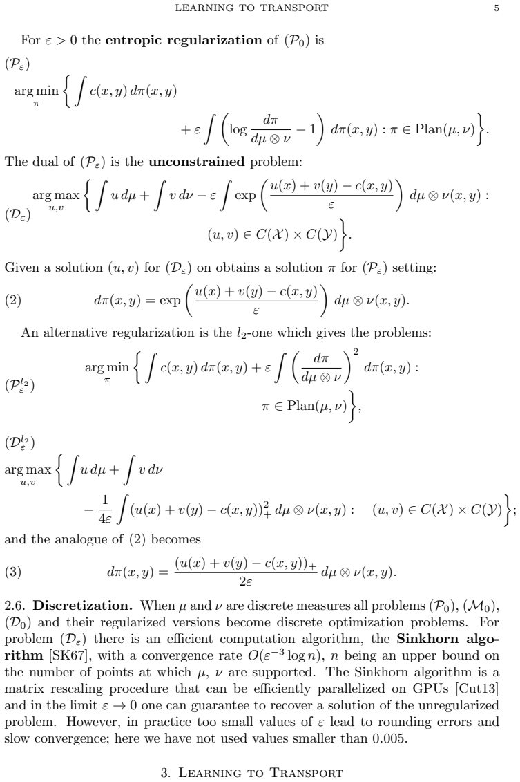
The load-bearing object is the benchmark itself: a planar pair of measures chosen so that the optimal transport map is non-smooth, because the target distribution is four separated disks. The evaluation is the mean squared distance from each learned map to a ground-truth optimal map, defined by running the Sinkhorn matrix-scaling algorithm on 1000 samples with entropic regularization $\varepsilon = 10^{-2}$. Around that target, the paper organizes the methods: flow Lagrangians that match means and covariances, Gaussian bumps, or $k$-nearest-neighbor discrepancies; adversarial min-max training; neural parametrizations of the entropic and $\ell^2$ regularized duals; and supervised regression of potentials, plans, or maps onto batch-wise Sinkhorn outputs.

What would settle it

Rerun the benchmark with several regularization levels (for example $\varepsilon = 10^{-1}, 10^{-2}, 10^{-3}$) and with an exactly solvable quadratic-cost pair where the true Monge map is known; if the relative ranking of the well-performing methods shifts with $\varepsilon$, the paper's conclusion depends on its chosen ground truth rather than on the methods themselves.

Watch

Extended reading notes

Core claim

The paper's claim, on its own terms, is that the choice among several algorithms for learning an optimal map matters less than their training stability. On the test problem—uniform mass on the unit disk moved to four disks centered at $(\pm 1,\pm 1)$, so the optimum requires splitting mass—the best flow, the supervised map and potential learners, and the entropic and $\ell^2$ regularized-dual parametrization all reach mean squared errors around $0.15$–$0.18$ relative to a Sinkhorn-defined target, while adversarial methods bottom out around $0.37$ or worse and show collapse. The paper further claims that learning the map directly, or distilling it from Sinkhorn on minibatches, is faster than the two-stage route of learning potentials first.

Load-bearing premise

The whole comparison rests on treating the Sinkhorn solution with entropic regularization $\varepsilon = 10^{-2}$ as the true optimal map; if that regularized map is far from the unregularized one, the reported errors and rankings could change.

Editorial extensions

If this is right

Supervised learning against Sinkhorn-computed minibatch solutions yields maps as good as solving the regularized dual, while avoiding a second fitting step when the map is learned directly.
Adversarial training should not be the default choice for neural optimal maps: on this problem it collapses mass inside the target support and its quality depends strongly on the penalty weight.
Flow heuristics that match local Gaussian bumps are competitive with mathematically grounded dual methods, so heuristic flows deserve a place in the toolset despite lacking guarantees.
When wall-clock time matters, methods that directly learn the map, such as the cost-regularized Gaussian-bump flow and the supervised map learner, are the cheapest among the well-performing options.

Reading between the lines

Editorial extensions of the paper, not claims the author makes directly.

If the pattern generalizes, the bottleneck in learning transport maps is optimization stability rather than model expressivity; a test on a higher-dimensional problem would show whether the benchmark's conclusions carry over.
The paper's ground truth is itself entropically regularized, so method rankings could depend on $\varepsilon$; rerunning the comparison at several $\varepsilon$ values, including a case with an analytic Monge map, would separate method quality from target blur.
A natural extension of the supervised route is to generate Sinkhorn labels in parallel and train the map network offline on streamed batches, which the paper's timing results suggest would be cheap.

Share X Bluesky LinkedIn Reddit HN

Signed reviews

No signed human review yet.

Editorial analysis

A structured set of objections, weighed in public.

Desk editor's note, referee report, and a circularity audit.

Desk Editor's Note

read the letter

Short version: this is a sincere empirical sweep of neural OT methods, with two genuinely new pieces—neural parametrization of dynamic flows and supervised distillation of Sinkhorn outputs. But the evaluation leans on a Sinkhorn 'ground truth' at ε=1e-2 that is never validated against the unregularized Monge map, and the supervised methods are trained on that same target. That makes the headline 'several methods yield similarly good maps' only as solid as that approximation, and the paper does not test it.

What's good: The paper tries many baselines (flows with covariance/Gaussian bumps/discrepancy, adversarial, dual, supervised) on a deliberately non-smooth 2D problem, reports convergence curves and timing, and is careful about initialization and normalization. The supervised-map variant is a reasonable idea, and the observation that Sinkhorn iterations per batch are faster than full dual training is useful. The writing is straightforward and notes the lack of theoretical guarantees.

Soft spots: (1) The ground truth is a conditional barycenter from the entropic plan, not the Monge map; for the quadratic cost with non-smooth support, the former smears mass near discontinuities. The paper gives no ε-sensitivity check. (2) The error bars σ(ε²) are across snapshots of one run, not across seeds; there are no repeated runs, so stability statements are anecdotal. (3) The supervised methods are trained to imitate Sinkhorn and then scored against Sinkhorn, which is a real circularity for those methods; the flows/adversarial methods at least are not trained on the target, but their score still depends on that target's validity. (4) The code URL is malformed (spaces), which can't be fixed by guessing; that is a blocker for reproducibility.

Overall, the comparison is plausible but not conclusive. The single 2D dataset is fine as a first test, but the missing convergence study in ε is the main experimental gap. I'd send it to review, but ask for a sensitivity analysis (ε smaller if feasible, or comparison to a semi-discrete OT solver) and at least a few seeds.

Who it's for: practitioners choosing among neural OT methods, and researchers working on supervised approaches to transport. It's not a foundational result, but it is a useful datapoint. I would not cite it for the rankings, but the supervised distillation idea might be worth citing in a related paper.

Referee Report

3 major / 5 minor

Summary. The paper compares several neural-network approaches for learning an optimal transport map between probability distributions, dividing them into heuristics (flow-based and adversarial training) and approaches with stronger mathematical motivation (regularized duals à la Seguy et al. and supervised learning from Sinkhorn outputs). The experiments use a single 2D benchmark where the source is uniform on the unit ball and the target is uniform on four disjoint balls, so the true optimal map is non-smooth. The evaluation metric (Eq. 12) compares each learned map against a ground truth Topt computed by Sinkhorn with entropic regularization ε = 10^-2 on 1000 samples. The main reported findings are that Gaussian-bump flows (tp exp), supervised learning of potentials or maps, and the dual formulation of [SDF+18] all achieve similar low errors, while adversarial training underperforms and is unstable.

Significance. If the results hold, the paper provides a useful practical comparison and lends support to the idea that supervised distillation from Sinkhorn is a viable path to learning transport maps, while also showing that the choice of method matters less than having a stable training procedure. The paper is accompanied by public code, and the visual inspection of maps in addition to a scalar metric is a strength. However, the significance is limited by the reliance on a single, low-dimensional synthetic benchmark and, more importantly, by the use of an entropically regularized Sinkhorn solution as the 'ground truth' optimal map, which makes the quantitative rankings and the central claim about producing 'good optimal maps' contingent on an unverified approximation.

major comments (3)

[§4.2, Eq. (12) and §4.1] The ground truth Topt is computed by Sinkhorn with entropic regularization ε = 10^-2, but the entropic optimal plan does not coincide with the unregularized Monge map for the quadratic cost. For a benchmark deliberately chosen to have a non-smooth optimal map, the entropic map Topt(x) = E_{π_ε}[Y|X] is a conditional barycenter and will differ from the hard assignment of the true optimal map, likely most severely near the discontinuities of Topt. The paper reports no sensitivity analysis with respect to ε (and states in §2.6 that values below 0.005 are impractical). Since every reported error and the conclusion in §4.7 that several methods produce 'similar good optimal maps' are measured against this target, the central quantitative claim is unsupported unless the entropic map is shown to be close to the true Monge map. A concrete fix is to compute an exact semi-discrete optimal map for this simple 2D problem and to report errors against that, or at least to provide an ε-sweep showing that the rankings are stable.
[§3.6 and Eq. (12)] The supervised methods are trained to imitate Sinkhorn outputs ('source of truth' in §3.6) and then evaluated against a Sinkhorn-based ground truth in Eq. (12). This creates a partial circularity: low ε² for supervised dual and supervised map partly measures fidelity to the same entropic algorithm used to generate the training labels, rather than accuracy relative to the true optimal map. The claim in §4.7 that supervised distillation from Sinkhorn is a viable path is therefore weakened. To break the circularity, the evaluation should use an independent ground truth (e.g., the exact semi-discrete Monge map) or at least report the unregularized transport cost of the learned maps against the true optimal value.
[§4.2, Tables 4.1–4.3] The reported ε² is the minimum over the S snapshot iterations, and σ(ε²) is computed only over iterations after tmin. This selection rule favors methods with high variance, because for a noisy training trajectory the minimum over snapshots can be substantially lower than the final or typical performance. For instance, supervised methods have σ(ε²) values around 0.08–0.10, much larger than tp exp (0.013), yet they are reported as achieving comparable ε². The conclusion that the methods 'yield similar good optimal maps' may thus be an artifact of the minimum-over-trajectory protocol. The paper should report final errors, medians, or use a proper validation-based model selection, and discuss how the rankings change.

minor comments (5)

[§3.1] Typo: 'assume taht T has been learned' should read 'assume that T has been learned'.
[§4.2] Equations (11) and (12) both use the symbol ε²; Eq. (11) is an integral over X while Eq. (12) is an empirical average. Using different symbols or explicit subscripts would improve clarity.
[§4.5, Table 4.3] The model names such as 'supervised map iters 1000 0.05' are described only in the surrounding text, and the table does not specify what 'iters' and the trailing number mean (number of Sinkhorn iterations and regularization coefficient, presumably). Adding a caption or footnote would make the table self-contained.
[§3.4] The statement that the inner max over θ in (Adv) 'would give +∞ if Tw#µ ≠ ν' is imprecise: it requires a universal function class (e.g., all 1-Lipschitz functions) and fails for finite neural networks. The authors themselves later note uncertainty about whether the adversarial term approximates a Wasserstein distance; the earlier sentence should be qualified.
[References] Reference [LA08] lists the authors as 'Giuseppe Savare Luigi Ambrosio, Nicola Giglio', which appears to be an error; the book is by Ambrosio, Gigli, and Savaré. The reference would benefit from correction.

Circularity Check

1 steps flagged · score 4.0 of 10

Supervised methods are trained on Sinkhorn labels and scored against a Sinkhorn-computed Topt, making their low error partly self-referential; the cross-method comparison retains independent content.

fitted input called prediction [Section 3.6 (supervised learning) and Section 4.2, Eq. (12) (performance benchmark)]
"An alternative approach to [SDF+18] is to use (Dε) as a “source of truth” to generate a stream of training data. [...] To define Topt we take samples {Xi}B i=1 ∼ µ, {Yj}B j=1 ∼ ν (B = 1000 in our experiments) and compute a “ground truth” Topt using the Sinkhorn algorithm with a low value of the entropic regularization (i.e. we set ε = 10−2 in (Pε) in our experiments)."

The supervised learning family is trained to approximate Sinkhorn-generated targets (potentials, plans, or maps) on minibatches, while the evaluation metric Eq. (12) measures mean squared distance to a Topt defined by the same Sinkhorn algorithm. Consequently, the low ε2 reported for “supervised dual” and “supervised map” is largely a measure of how well the neural networks can imitate the same procedure that defines the benchmark, rather than an independent confirmation that the maps are optimal for the unregularized cost. The circularity is partial: the training labels use ε = 0.05 while the evaluation Topt uses ε = 0.01, and the flow and adversarial methods are not trained on Sinkhorn labels, so the ranking among methods retains independent content.

full rationale

The paper is an empirical benchmark rather than a formal derivation: no theorem equates the proposed methods with their inputs, and there are no load-bearing self-citations. The only substantial circular thread is that Sinkhorn is used both as the label generator for supervised training (Section 3.6) and as the ground-truth oracle in the evaluation metric (Section 4.2, Eq. 12). For the supervised family, low error is partially forced by construction, since the networks are trained to reproduce Sinkhorn outputs and then scored against a Sinkhorn output. This does not invalidate the central comparison: flows using Gaussian bumps, dual methods, and adversarial models are evaluated against the same external Sinkhorn reference without being trained on it, and the supervised training/evaluation Sinkhorn parameters differ (0.05 vs 0.01). The concern that entropic regularization at ε = 10−2 may differ from the unregularized Monge map is a correctness/validity issue, not a circularity, and should be reported separately. Overall, one partial circularity is present, but the headline claim still has independent empirical content.

Assumptions & free parameters 3 free parameters · 4 assumptions · 0 invented entities

The paper introduces no new physical or mathematical entities. Its central claims rest on the assumption that Sinkhorn with low epsilon gives a valid ground-truth map, that neural networks have sufficient capacity, and that the chosen hyperparameters are representative.

free parameters (3)

Entropic regularization epsilon for ground truth = 0.01
Used to compute Topt in Eq. (12), the reference optimal map. The choice affects every reported error; no sensitivity analysis is provided.
Number of Gaussian bumps K = not stated explicitly
In the exp and tp exp flows, the family {f_k} is a grid of Gaussian bumps; K and sigma^2 are hand chosen before training and affect the flow's behavior.
Gaussian width sigma^2 = not stated
Width of the Gaussian bumps in Eq. (8), chosen by hand.

assumptions (4)

domain assumption Existence and regularity of optimal transport map T
Section 3.2 states 'we deliberately neglect issues about the existence and regularity of such T', assuming an optimal Monge map exists for the considered measures.
ad hoc to paper Sinkhorn with epsilon=1e-2 approximates the true optimal map
Section 4.2 defines Topt via Sinkhorn with epsilon=1e-2; this is the benchmark for all comparisons.
domain assumption Neural networks can represent the optimal map and potentials
Section 3.1 states that even two hidden layers can represent rich spaces of nonlinear functions; the methods rely on this capacity.
domain assumption Stochastic gradient descent converges to a good solution
All methods train via stochastic gradient descent; convergence is not proved.

how reviews work

0 comments

Cite this review

Pith. "Pith review of Learning to Transport with Neural Networks." pith.science (2026). https://pith.science/paper/YFJ7YG5E

@misc{pith2026190801394,
  author       = {Pith},
  title        = {Pith review of: Learning to Transport with Neural Networks},
  year         = {2026},
  howpublished = {\url{https://pith.science/paper/YFJ7YG5E}},
  note         = {Machine review of arXiv:1908.01394}
}

read the original abstract

We compare several approaches to learn an Optimal Map, represented as a neural network, between probability distributions. The approaches fall into two categories: ``Heuristics'' and approaches with a more sound mathematical justification, motivated by the dual of the Kantorovitch problem. Among the algorithms we consider a novel approach involving dynamic flows and reductions of Optimal Transport to supervised learning.

Figures

Figures reproduced from arXiv: 1908.01394 by the authors.

**Figure 3.1.** Different approaches to learn an Optimal Map 3.1. Representations. What is a good way to represent mathematical objects like µ, ν, T, u or v? The answer will likely depend on the setting. For example µ and ν can be discretized on a fixed mesh and then one needs to keep track of the value of maps and functions only on a fixed set of points. As observed in [TT16] mesh-based approaches do not scale well in the dimensio… view at source ↗

**Figure 4.1.** Visualization of µ, ν with 1024 samples t 7→ t/T to compare the convergence rate across the iterations. Once we single out promising algorithms we are able to dig more into the training times using statistics that we log at periodic intervals in Tensorboard. Finally, for each of the S timesteps we save an image of the map Tw(s) , see for example figure 4.2. At the end of training we compose the images into a movie (… view at source ↗

Figures from the paper (25 more)

**Figure 4.2.** Figure 4.2: Example of a “movie frame” generated during training. Blue points are sampled from µ, and black ones from ν. Red points are the images of each blue point under Tw(t) and we keep them linked to their “source point” via a black segment. • covariance: We try to force m…

**Figure 4.5.** Figure 4.5: We observe a quick chaotic push to collapse [PITH_FULL_IMAGE:figures/full_fig_p012_4_5.png]

**Figure 4.3.** Figure 4.3: The final transport yielded by tp covariance µ into the support of ν while keeping the shapes of T#µ and ν comparable, see [PITH_FULL_IMAGE:figures/full_fig_p013_4_3.png]

**Figure 4.10.** Figure 4.10: The flows based on exp give the best results and greatly benefit from adding the regularization. The algorithm exp reaches the minimum after about 30% of the iterations while tp exp does not improve substantially after 60% of the iterations, see [PITH_FULL_IMAGE:fi…

**Figure 4.4.** Figure 4.4: Convergence rate for covariance and tp covariance [PITH_FULL_IMAGE:figures/full_fig_p014_4_4.png]

**Figure 4.6.** Figure 4.6: Collapse of transport map for discr 5, t = 8000 [PITH_FULL_IMAGE:figures/full_fig_p015_4_6.png]

**Figure 4.7.** Figure 4.7: Convergence rate for tp discr 1 and tp discr 5 In [PITH_FULL_IMAGE:figures/full_fig_p015_4_7.png]

**Figure 4.8.** Figure 4.8: Collapse of transport map for tp discr 5, t = 7800 [PITH_FULL_IMAGE:figures/full_fig_p016_4_8.png]

**Figure 4.9.** Figure 4.9: Convergence for the flows based on symdiscr @ N Also increasing the number of iterations of the adversarial network leaves it stuck at a point with a higher value of ε2. The best model is adv l1 2 which reaches the minimal ε2 at around 75% of the iterations. However,…

**Figure 4.11.** Figure 4.11: Convergence for the flows exp, tp exp of ν, see [PITH_FULL_IMAGE:figures/full_fig_p017_4_11.png]

**Figure 4.12.** Figure 4.12: Transport map for exp, t = 9000 [PITH_FULL_IMAGE:figures/full_fig_p018_4_12.png]

**Figure 4.13.** Figure 4.13: Transport map for tp exp, t = 5400 constant while the cost component increases. The first phase corresponds to the adversarial loss starting to discriminate between µ and ν and the second phase to the cost increasing as µ starts to move towards ν [PITH_FULL_IMAGE:f…

**Figure 4.14.** Figure 4.14: Convergence for the “adversarial” models 4.5. Comparison of Approaches based on duals & supervised learning. In table 4.3 we can see a comparison of the performances of the algorithms based on the dual methods of Subsection 3.5 and supervised learning of Subsection …

**Figure 4.15.** Figure 4.15: Chaotic behavior of adversarial training for λ = 100 at iterations t = 1000, 8000, 36000 (from left to right) [PITH_FULL_IMAGE:figures/full_fig_p020_4_15.png]

**Figure 4.16.** Figure 4.16: Transport map for adv l1 2, t = 39000 j). However the equations in the original paper [SDF+18, Alg. 1] suggest to use a double sum for the regularization term. While taking the sum degrades a bit the entropic model, it has a positive effect on the l2-regularized mod…

**Figure 4.17.** Figure 4.17: Comparison of the cost and adversarial component of the loss for adv l1 2 across the training steps. Note we use statistics in TensorBoard so we are not restricted to the S snapshots. the end of the training T#µ becomes too diffused, see [PITH_FULL_IMAGE:figures/f…

**Figure 4.23.** Figure 4.23: Finally, we point out that the approach based on directly learning [PITH_FULL_IMAGE:figures/full_fig_p021_4_23.png]

**Figure 4.18.** Figure 4.18: Comparison of the final maps using the dual approach with l2-regularization; on the left using the mean aggregation and on the right the sum. In general, total timings are relatively comparable. However, we see the advantage of using models like tp exp or supervi…

**Figure 4.19.** Figure 4.19: Convergence rate of models based on the dual approach [PITH_FULL_IMAGE:figures/full_fig_p023_4_19.png]

**Figure 4.20.** Figure 4.20: Comparison of the final maps for seguy l2 sum 0.1 (left) and seguy ent mean 0.1 (right). 4.7. Conclusion. We have compared a variety of approaches to find an optimal map between probability distributions. We find that, despite different theoretical/heuristic justifi…

**Figure 4.21.** Figure 4.21: Convergence rate of models based on the supervised [PITH_FULL_IMAGE:figures/full_fig_p024_4_21.png]

**Figure 4.22.** Figure 4.22: Poor quality of transport maps for supervised prob, left at t = 1k and right at t = 47k. References [AB17] Martin Arjovsky and L´eon Bottou. Towards Principled Methods for Training Generative Adversarial Networks. arXiv e-prints, page arXiv:1701.04862, Jan 2017. [A…

Discussion (0). Continue with ORCID to comment.

Reference graph

Works this paper leans on

21 extracted references · 15 canonical work pages

[1]

Towards Principled Methods for Training Generative Adversarial Networks

Martin Arjovsky and L \'e on Bottou . Towards Principled Methods for Training Generative Adversarial Networks . arXiv e-prints , page arXiv:1701.04862, Jan 2017

arXiv 2017
[2]

Wasserstein GAN

Martin Arjovsky , Soumith Chintala , and L \'e on Bottou . Wasserstein GAN . arXiv e-prints , page arXiv:1701.07875, Jan 2017

arXiv 2017
[3]

Sinkhorn distances: Lightspeed computation of optimal transport

Marco Cuturi. Sinkhorn distances: Lightspeed computation of optimal transport. In Proceedings of the 26th International Conference on Neural Information Processing Systems - Volume 2 , NIPS'13, pages 2292--2300, USA, 2013. Curran Associates Inc

work page 2013
[4]

Stochastic optimization for large-scale optimal transport

Aude Genevay, Marco Cuturi, Gabriel Peyr \'e , and Francis Bach. Stochastic optimization for large-scale optimal transport. In Proceedings of the 30th International Conference on Neural Information Processing Systems , NIPS'16, pages 3440--3448, USA, 2016. Curran Associates Inc

work page 2016
[5]

Multiscale Strategies for Computing Optimal Transport

Samuel Gerber and Mauro Maggioni. Multiscale strategies for computing optimal transport. CoRR , abs/1708.02469, 2017

work page Pith review arXiv 2017
[6]

Generative adversarial nets

Ian Goodfellow, Jean Pouget-Abadie, Mehdi Mirza, Bing Xu, David Warde-Farley, Sherjil Ozair, Aaron Courville, and Yoshua Bengio. Generative adversarial nets. In Z. Ghahramani, M. Welling, C. Cortes, N. D. Lawrence, and K. Q. Weinberger, editors, Advances in Neural Information Processing Systems 27 , pages 2672--2680. Curran Associates, Inc., 2014

2014
[7]

Shunmuga Krishnan and Ramesh K

S. Shunmuga Krishnan and Ramesh K. Sitaraman. Video stream quality impacts viewer behavior: Inferring causality using quasi-experimental designs. In Proceedings of the 2012 Internet Measurement Conference , IMC '12, pages 211--224, New York, NY, USA, 2012. ACM

work page 2012
[8]

From word embeddings to document distances

Matt Kusner, Yu Sun, Nicholas Kolkin, and Kilian Weinberger. From word embeddings to document distances. In Francis Bach and David Blei, editors, Proceedings of the 32nd International Conference on Machine Learning , volume 37 of Proceedings of Machine Learning Research , pages 957--966, Lille, France, 07--09 Jul 2015. PMLR

work page 2015

Show all 21 references

[9]

Gradient Flows In Metric Spaces and in the Space of Probability Measures

Giuseppe Savare Luigi Ambrosio, Nicola Giglio. Gradient Flows In Metric Spaces and in the Space of Probability Measures . Birkhäuser Basel, 2008. Available at: http://www2.stat.duke.edu/ sayan/ambrosio.pdf

2008
[10]

Ricci curvature for metric-measure spaces via optimal transport

John Lott and Cédric Villani. Ricci curvature for metric-measure spaces via optimal transport. Annals of Mathematics , 169(3):903--991, 2009

2009
[11]

Quasi experimentation at netflix

Netflix. Quasi experimentation at netflix. https://medium.com/netflix-techblog/quasi-experimentation-at-netflix-566b57d2e362. Technology Blog (Sep 2018), Accessed at: 2019-07-30

2018
[12]

Orlova, Noah Zimmerman, Stephen Meehan, Connor Meehan, Jeffrey Waters, Eliver E

Darya Y. Orlova, Noah Zimmerman, Stephen Meehan, Connor Meehan, Jeffrey Waters, Eliver E. B. Ghosn, Alexander Filatenkov, Gleb A. Kolyagin, Yael Gernez, Shanel Tsuda, Wayne Moore, Richard B. Moss, Leonore A. Herzenberg, and Guenther Walther. Earth mover’s distance (emd): A tru...

2016
[13]

Computational optimal transport

Gabriel Peyré and Marco Cuturi. Computational optimal transport. Foundations and Trends® in Machine Learning , 11(5-6):355--607, 2019

2019
[14]

Sinkhorn AutoEncoders

Giorgio Patrini , Rianne van den Berg , Patrick Forr \'e , Marcello Carioni , Samarth Bhargav , Max Welling , Tim Genewein , and Frank Nielsen . Sinkhorn AutoEncoders . arXiv e-prints , page arXiv:1810.01118, Oct 2018

2018 arXiv
[15]

Optimal Transport for Applied Mathematicians

Filippo Santambrogio. Optimal Transport for Applied Mathematicians . Birkhäuser Basel, 2015. Available at: https://www.math.u-psud.fr/ filippo/OTAM-cvgmt.pdf

2015
[16]

Large-scale optimal transport and mapping estimation

Vivien Seguy, Bharath Bhushan Damodaran, R \'e mi Flamary, Nicolas Courty, Antoine Rolet, and Mathieu Blondel. Large-scale optimal transport and mapping estimation. In Proceedings of the International Conference in Learning Representations , 2018

2018
[17]

Convolutional wasserstein distances: Efficient optimal transportation on geometric domains

Justin Solomon, Fernando de Goes, Gabriel Peyr \'e , Marco Cuturi, Adrian Butscher, Andy Nguyen, Tao Du, and Leonidas Guibas. Convolutional wasserstein distances: Efficient optimal transportation on geometric domains. ACM Trans. Graph. , 34(4):66:1--66:11, July 2015

2015
[18]

Concerning nonnegative matrices and doubly stochastic matrices

Richard Sinkhorn and Paul Knopp. Concerning nonnegative matrices and doubly stochastic matrices. Pacific J. Math. , 21(2):343--348, 1967

1967
[19]

Giulio Trigila and Esteban G. Tabak. Data-driven optimal transport. Communications on Pure and Applied Mathematics , 69(4):613--648, 2016

2016
[20]

Sharp asymptotic and finite-sample rates of convergence of empirical measures in Wasserstein distance

Jonathan Weed and Francis Bach . Sharp asymptotic and finite-sample rates of convergence of empirical measures in Wasserstein distance . arXiv e-prints , page arXiv:1707.00087, Jun 2017

2017 arXiv
[21]

Energy-based Generative Adversarial Network

Junbo Zhao , Michael Mathieu , and Yann LeCun . Energy-based Generative Adversarial Network . arXiv e-prints , page arXiv:1609.03126, Sep 2016

2016 arXiv

Pith tools

Reviewed August 14, 2026 · model on record in the stance chip above.

[1] [1]

Towards Principled Methods for Training Generative Adversarial Networks

Martin Arjovsky and L \'e on Bottou . Towards Principled Methods for Training Generative Adversarial Networks . arXiv e-prints , page arXiv:1701.04862, Jan 2017

arXiv 2017

[2] [2]

Wasserstein GAN

Martin Arjovsky , Soumith Chintala , and L \'e on Bottou . Wasserstein GAN . arXiv e-prints , page arXiv:1701.07875, Jan 2017

arXiv 2017

[3] [3]

Sinkhorn distances: Lightspeed computation of optimal transport

Marco Cuturi. Sinkhorn distances: Lightspeed computation of optimal transport. In Proceedings of the 26th International Conference on Neural Information Processing Systems - Volume 2 , NIPS'13, pages 2292--2300, USA, 2013. Curran Associates Inc

work page 2013

[4] [4]

Stochastic optimization for large-scale optimal transport

Aude Genevay, Marco Cuturi, Gabriel Peyr \'e , and Francis Bach. Stochastic optimization for large-scale optimal transport. In Proceedings of the 30th International Conference on Neural Information Processing Systems , NIPS'16, pages 3440--3448, USA, 2016. Curran Associates Inc

work page 2016

[5] [5]

Multiscale Strategies for Computing Optimal Transport

Samuel Gerber and Mauro Maggioni. Multiscale strategies for computing optimal transport. CoRR , abs/1708.02469, 2017

work page Pith review arXiv 2017

[6] [6]

Generative adversarial nets

Ian Goodfellow, Jean Pouget-Abadie, Mehdi Mirza, Bing Xu, David Warde-Farley, Sherjil Ozair, Aaron Courville, and Yoshua Bengio. Generative adversarial nets. In Z. Ghahramani, M. Welling, C. Cortes, N. D. Lawrence, and K. Q. Weinberger, editors, Advances in Neural Information Processing Systems 27 , pages 2672--2680. Curran Associates, Inc., 2014

2014

[7] [7]

Shunmuga Krishnan and Ramesh K

S. Shunmuga Krishnan and Ramesh K. Sitaraman. Video stream quality impacts viewer behavior: Inferring causality using quasi-experimental designs. In Proceedings of the 2012 Internet Measurement Conference , IMC '12, pages 211--224, New York, NY, USA, 2012. ACM

work page 2012

[8] [8]

From word embeddings to document distances

Matt Kusner, Yu Sun, Nicholas Kolkin, and Kilian Weinberger. From word embeddings to document distances. In Francis Bach and David Blei, editors, Proceedings of the 32nd International Conference on Machine Learning , volume 37 of Proceedings of Machine Learning Research , pages 957--966, Lille, France, 07--09 Jul 2015. PMLR

work page 2015