Geometry and localization: Probing Localization Landscape Theory on the Bethe Lattice
Pith reviewed 2026-06-29 00:00 UTC · model grok-4.3
The pith
The LLT percolation transition on the Bethe lattice follows standard mean-field universality while the Anderson transition does not.
A machine-rendered reading of the paper's core claim, the machinery that carries it, and where it could break.
Core claim
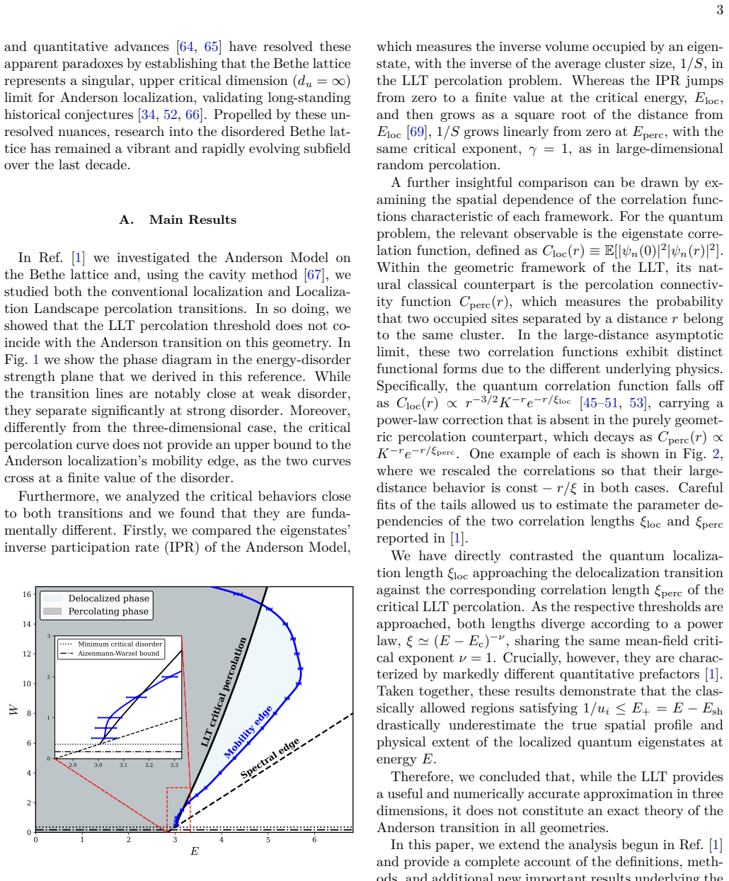
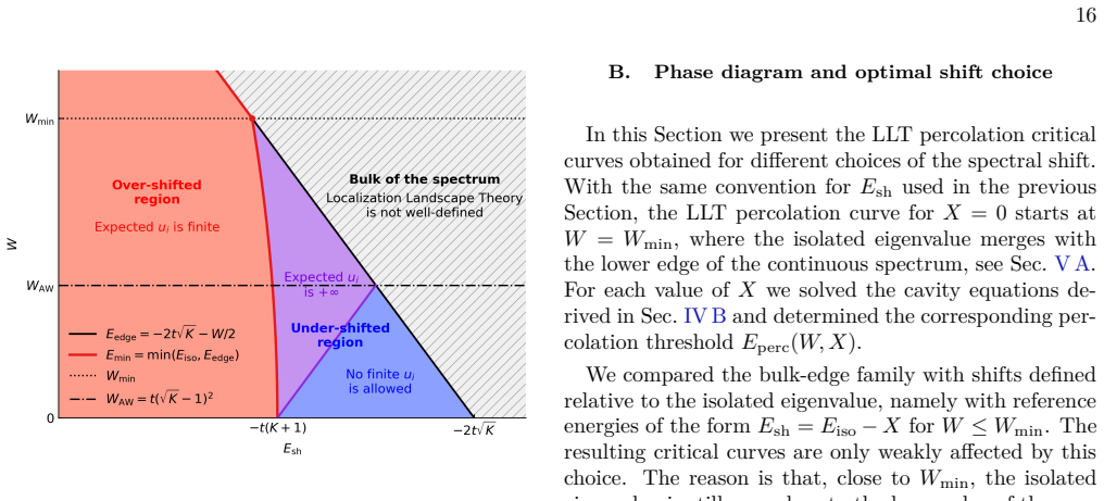
On the Bethe lattice the LLT percolation transition falls into the standard mean-field universality class in sharp contrast with the unconventional critical behavior of the Anderson transition. The LLT framework reproduces several exact results in the very low-disorder regime: it predicts the position of the isolated eigenvalue, the minimal disorder at which both the LLT percolation curve and the mobility edge first appear, and the Aizenman-Warzel lower bound for localization. It also overestimates the amplitude of the density-of-states tails close to the boundary of the continuous spectrum.
What carries the argument
Exact solvability of the Anderson model and the LLT percolation problem on the Bethe lattice, allowing direct comparison of their critical behaviors.
If this is right
- LLT does not generally reproduce the quantum critical properties of Anderson localization.
- LLT remains useful for predicting features of the very low-disorder regime.
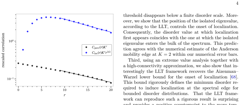
- The LLT prediction for the density of states overestimates the amplitude of the tails near the boundary of the continuous spectrum.
- The dependence of the LLT percolation threshold on energy shift can be evaluated exactly.
Where Pith is reading between the lines
- Numerical agreement between LLT and Anderson localization observed in three dimensions may be limited to the low-disorder regime rather than the critical point.
- Geometric interpretations of localization may require additional corrections to capture unconventional critical behavior on tree-like structures.
- Extreme-value statistics of the variables controlling LLT could be tested on other exactly solvable graphs.
Load-bearing premise
The Bethe lattice permits exact, directly comparable solutions for both the Anderson model and the LLT percolation problem.
What would settle it
A direct computation of the critical exponents for the LLT percolation threshold on the Bethe lattice that either matches or deviates from the known unconventional exponents of the Anderson transition.
Figures
read the original abstract
The Localization Landscape Theory (LLT) offers a classical analogy for understanding Anderson localization through an effective confining potential, whose percolation threshold has been proposed to mark the mobility edge. While this correspondence shows striking numerical agreement in three dimensions, its theoretical foundations remain an open question. In this work, we extend the analysis of the LLT on the Bethe lattice presented in~\cite{Tonetti2026}. In this setting in both the Anderson localization transition and the LLT percolation problem admit exact solutions. Our analysis reveals that the two transitions are distinct, with markedly different critical behaviors. Notably, the LLT percolation transition falls into the standard mean-field universality class, in sharp contrast with the unconventional critical behavior of the Anderson transition on the Bethe lattice. Nonetheless, the LLT framework reproduces several exact results, capturing nontrivial features of the very low-disorder regime: it predicts the position of the isolated eigenvalue, the minimal disorder at which both the LLT percolation curve and the mobility edge first appear, and the Aizenman--Warzel lower bound for localization. We also study the dependence of the LLT percolation threshold on the energy shift, evaluate the LLT prediction for the Density of States, and derive several results on the statistical properties of the variables controlling the problem. Finally, we develop an extreme-value analysis showing that the LLT prediction for the Density of States overestimates the amplitude of the tails close to the boundary of the continuous spectrum. These findings provide an exact analytical benchmark showing that, despite its geometric appeal, the LLT does not generally reproduce the quantum critical properties of Anderson localization, while still offering a powerful tool to understand its very low-disorder regime.
Editorial analysis
A structured set of objections, weighed in public.
Referee Report
Summary. The manuscript extends prior analysis of Localization Landscape Theory (LLT) on the Bethe lattice, where both the Anderson localization transition and LLT percolation admit exact solutions. It demonstrates that the transitions are distinct, with LLT percolation belonging to the standard mean-field universality class in contrast to the unconventional critical behavior of the Anderson transition. LLT is shown to reproduce several exact low-disorder results, including the isolated eigenvalue position, the minimal disorder at which percolation and the mobility edge appear, and the Aizenman-Warzel bound, while also examining energy-shift dependence, the LLT density-of-states prediction, statistical properties of controlling variables, and an extreme-value analysis indicating overestimation of DOS tails near the continuous spectrum boundary.
Significance. If the exact solutions and comparisons hold, the work supplies a valuable analytical benchmark on a solvable model, clarifying that LLT captures nontrivial low-disorder features of Anderson localization but does not reproduce its quantum critical properties. The parameter-free exact derivations, direct comparison of critical behaviors, and falsifiable predictions for the DOS tails constitute clear strengths.
minor comments (2)
- [Abstract] The citation to Tonetti2026 in the abstract and introduction should include the full reference details and a brief statement of which results are extended versus newly derived.
- Notation for the statistical variables controlling the LLT percolation problem could be introduced with a short table or explicit definitions early in the text to aid readers unfamiliar with the prior setup.
Simulated Author's Rebuttal
We thank the referee for their positive assessment of our manuscript, including the recognition of its exact solutions, comparisons of critical behaviors, and falsifiable predictions. We appreciate the recommendation to accept.
Circularity Check
Minor self-citation to prior setup; central claims rest on independent exact solutions and comparisons
full rationale
The manuscript extends the Bethe-lattice LLT setup introduced in the authors' cited prior work (Tonetti2026) but derives its core findings—the distinct universality classes of the LLT percolation transition (standard mean-field) versus the Anderson transition (unconventional), plus exact reproduction of the isolated eigenvalue, minimal disorder threshold, and Aizenman-Warzel bound—directly from the model's exact solvability and new statistical analysis. No derivation step reduces by construction to a fitted parameter, self-defined quantity, or load-bearing self-citation chain; the self-citation supplies only the lattice framework while the critical-behavior contrasts and low-disorder benchmarks are independently verifiable against the Bethe-lattice equations.
Axiom & Free-Parameter Ledger
axioms (1)
- domain assumption The Bethe lattice admits exact solutions for both the Anderson localization transition and the LLT percolation problem.
Forward citations
Cited by 1 Pith paper
-
Anderson localization on the Bethe lattice
Pedagogical review of the cavity equations, order parameter, and critical behavior for Anderson localization on the Bethe lattice.
Reference graph
Works this paper leans on
-
[1]
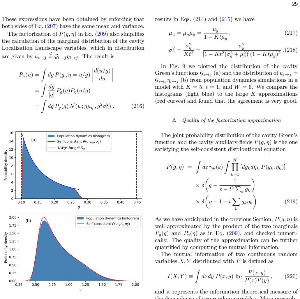
(209), and checked numeri- cally
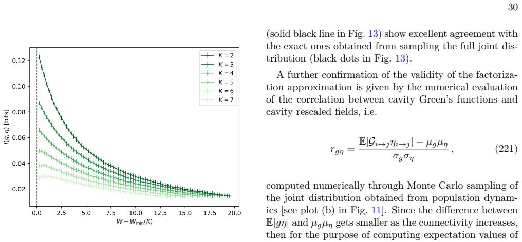
Quality of the factorization approximation The joint probability distribution of the cavity Green’s function and the cavity auxiliary fieldsP(g,η) is the one satisfying the self-consistent distributional equation P(g,η) = ∫ dεγ+(ε) ∫ K∏ k=1 [dgkdηk P(gk,ηk)] ×δ ( g− 1 ε−t2 ∑ kgk ) ×δ ( η−1−t ∑ k gkηk ) .(219) As we have anticipated in the previous Section...
-
[2]
Lower bound for the critical disorder and isolated eigenvalue It is important to note that, for physical consistency, the expectation value of the cavity rescaled fields must be non-negative, since the opposite would imply nega- tive Localization Landscape variables, which is impossi- ble, as explained in the End Matter of Ref. [1]. Therefore, Eqs. (214) ...
-
[3]
III D, we start from the self-consistent distributional equation (95)
Linear stability analysis Following the same idea of [44], and already used in the analysis of the Anderson problem in Sec. III D, we start from the self-consistent distributional equation (95). Using the integral representation of the Dirac delta 34 δ ( p−θ(gη−1/E+) ∑ k pk ) = ∫ ∞ −∞ dλ′ 2πe−iλ′(p−θ(gη−1/E+) ∑ kpk),(247) we can rewrite P(g,η,p) = ∫ dλ′ 2...
-
[4]
In the general case, a cluster consists of a connected component of lattice sitesiwhereu i≥1/E+
Divergence of the average cluster size An alternative method to determine the critical curve involves deriving an expression for the average cluster size Sand identifying the values (E,W) for whichSdiverges. In the general case, a cluster consists of a connected component of lattice sitesiwhereu i≥1/E+. The sta- tistical dependence betweenu i andu k (fork...
-
[5]
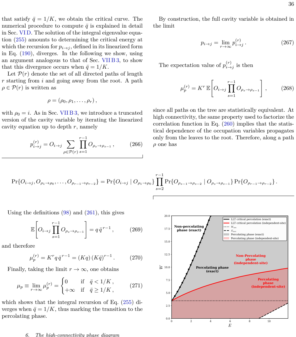
It displays both the curve de- rived from the independent-site approximation condition [Eq
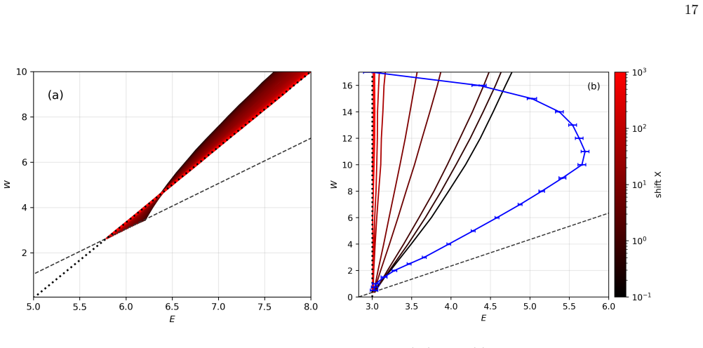
The high-connectivity phase diagram Figure 13 presents the phase diagram obtained in the high-connectivity limit. It displays both the curve de- rived from the independent-site approximation condition [Eq. (183)] for the edge-shift perscription (E sh(W) = Eedge(W)) and the one obtained using the exact crite- rion [Eq. (265)]. The phase diagram in Fig. 13 ...
-
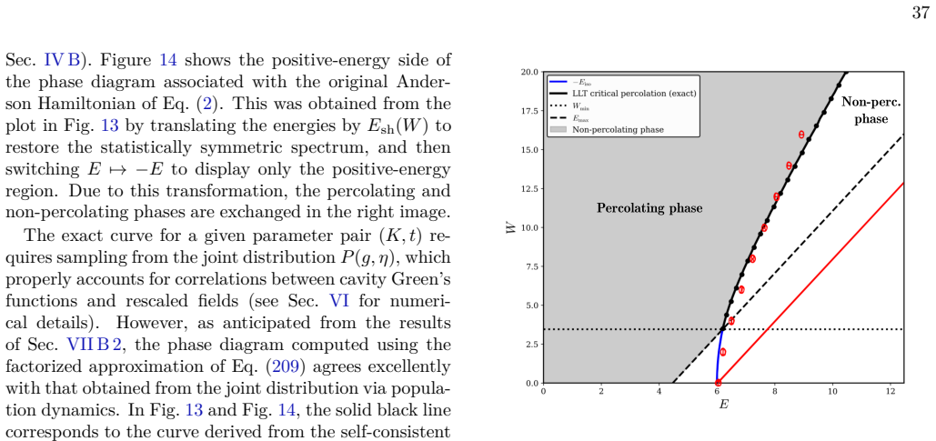
[6]
Hamiltonian with the statistically symmetric spectrum of Eq. (2). All the curves have been obtained from the ones in Fig. 13 by means of a translation and inversion of sign as explained in Sec. VII B 6. The independent-site critical curve has not been plotted as it loses its physical interpretation in the symmetric case. Red dots: Localization Landscape p...
-
[7]
Cavity Green’s functions’ marginal We consider the closed recursion of Eq. (51). As the cavity Green’s functions are real and positive, the denominator of Eq. (51) must always be positive, this means thatt 2 ∑ l∈∂k\iGl→k≤εi for any draw ofεk and {Gl→k}l∈∂k\ifrom their respective distributions. Since 38 the support of the distribution ofεk is bounded, it f...
-
[8]
Cavity rescaled fields’ marginal The probability density function of the cavity rescaled fields can have either bounded or unbounded support, depending on the value of the additional shiftX. In- deed, if the normal and cavity rescaled fields had finite upper bounds ˜MηandMη, respectively, then the coupled equations Mη= 1 +tKM gMη,(321) ˜Mη= 1 +t(K+ 1)M gM...
-
[9]
Localization Landscape variables’ marginal and effective potentials We now study the marginal distribution of the Local- ization Landscape variables. From Eq. (48) one has ui =G iiηi .(382) The diagonal Green’s functions are positive and bounded in the interval [˜mg, ˜Mg], where ˜Mg = 1 εmin−(K+ 1)t2Mg ,(383) ˜mg = 1 εmax−(K+ 1)t2mg .(384) HereM g, mg are...
-
[10]
Fondation CFM pour la recherche
Summary of the tail results We summarize here the main asymptotic results ob- tained for the right tails of the cavity Green’s functions, the rescaled fields, and the Localization Landscape vari- ables. First, the marginal distribution of the cavity Green’s functions is supported on a compact interval [mg,Mg]⊂ (0,+∞) in presence of an extra shiftX >0. Def...
-
[11]
L. Tonetti, L. F. Cugliandolo, and M.Tarzia,Testing the localization landscape theory(2026), arXiv:2512.04037
-
[12]
P. W. Anderson, Phys. Rev.109, 1492 (1958), URL https://doi.org/10.1103/PhysRev.109.1492
-
[13]
P. A. Lee and T. V. Ramakrishnan, Rev. Mod. Phys.57, 287 (1985), URLhttps://doi.org/10.1103/ RevModPhys.57.287
1985
-
[15]
Lagendijk, B
A. Lagendijk, B. A. van Tiggelen, and D. S. Wiersma, Phys. Today62, 24 (2009), URLhttps://doi.org/10. 1063/1.3206091
2009
-
[16]
Segev, Y
M. Segev, Y. Silberberg, and D. N. Christodoulides, Nat. Phot.7, 197 (2013), URLhttps://doi.org/10.1038/ nphoton.2013.30
2013
-
[17]
A. Aspect and M. Inguscio, Phys. Today62, 30 (2009), URLhttps://doi.org/10.1063/1.3206092
-
[18]
Roati, C
G. Roati, C. D’Errico, L. Fallani, M. Fattori, C. Fort, M. Zaccanti, G. Modugno, M. Modugno, and M. Ingus- cio, Nature453, 895 (2008), URLhttps://doi.org/10. 1038/nature07071
2008
-
[19]
J. Billy, V. Josse, Z. Zuo, A. Bernard, B. Hambrecht, P. Lugan, D. Cl´ ement, L. Sanchez-Palencia, P. Bouyer, and A. Aspect, Nature453, 891 (2008), URLhttps: //doi.org/10.1038/nature07000
-
[20]
Kondov, W
S. Kondov, W. McGehee, J. Zirbel, and B. DeMarco, Sci- 48 ence334, 66 (2011), URLhttps://doi.org/10.1126/ science.1209019
2011
-
[21]
F. Jendrzejewski, A. Bernard, K. Mueller, P. Cheinet, V. Josse, M. Piraud, L. Pezz´ e, L. Sanchez-Palencia, A. Aspect, and P. Bouyer, Nat. Phys.8, 398 (2012), URL https://doi.org/10.1038/nphys2256
-
[22]
G. Semeghini, M. Landini, P. Castilho, S. Roy, G. Spag- nolli, A. Trenkwalder, M. Fattori, M. Inguscio, and G. Modugno, Nat. Phys.11, 554 (2015), URLhttps: //doi.org/10.1038/nphys3339
-
[24]
H. Hu, A. Strybulevych, J. H. Page, S. E. Skipetrov, and B. A. van Tiggelen, Nat. Phys.4, 945 (2008), URL https://doi.org/10.1038/nphys1101
-
[25]
N. F. Mott and W. D. Twose, Adv. Phys.10, 107 (1961), URLhttps://doi.org/10.1080/00018736100101271
-
[26]
L. P. Gor’kov, A. I. Larkin, and D. E. Khmel’nitski˘ ı, Particle conductivity in a two-dimensional random poten- tial(World Scientific, 1996), pp. 157–161, URLhttps: //doi.org/10.1142/9789814317344_0022
-
[27]
E. Abrahams, P. W. Anderson, D. C. Licciardello, and T. V. Ramakrishnan, Phys. Rev. Lett.42, 673 (1979), URLhttps://doi.org/10.1103/PhysRevLett.42.673
-
[28]
B. Kramer and A. MacKinnon, Rep. Prog. Phys.56, 1469 (1993), URLhttps://doi.org/10.1088/0034-4885/56/ 12/001
-
[29]
F. Wegner, Z. Phys. B Cond. Matt.35, 207 (1979), URL https://doi.org/10.1007/BF01319839
-
[30]
A. W. W. Ludwig, Phys. Scripta2016, 014001 (2015), URLhttps://doi.org/10.1088/0031-8949/ 2015/T168/014001
-
[31]
P. W. Brouwer, C. Mudry, B. D. Simons, and A. Altland, Phys. Rev. Lett.81, 862 (1998), URLhttps://doi.org/ 10.1103/PhysRevLett.81.862
-
[32]
T. Senthil, M. P. A. Fisher, L. Balents, and C. Nayak, Phys. Rev. Lett.81, 4704 (1998), URLhttps://doi. org/10.1103/PhysRevLett.81.4704
-
[33]
I. A. Gruzberg, A. W. W. Ludwig, and N. Read, Phys. Rev. Lett.82, 4524 (1999), URLhttps://doi.org/10. 1103/PhysRevLett.82.4524
1999
-
[34]
Senthil, J
T. Senthil, J. B. Marston, and M. P. A. Fisher, Phys. Rev. B60, 4245 (1999), URLhttps://doi.org/10. 1103/PhysRevB.60.4245
1999
-
[35]
N. Read and D. Green, Phys. Rev. B61, 10267 (2000), URLhttps://doi.org/10.1103/PhysRevB.61.10267
-
[36]
M. Titov, P. W. Brouwer, A. Furusaki, and C. Mudry, Phys. Rev. B63, 235318 (2001), URLhttps://doi.org/ 10.1103/PhysRevB.63.235318
-
[37]
D. M. Basko, I. L. Aleiner, and B. L. Altshuler, Ann. Phys. (N. Y.)321, 1126 (2006), ISSN 0003, URLhttp: //dx.doi.org/10.1016/j.aop.2005.11.014
-
[38]
I. V. Gornyi, A. D. Mirlin, and D. G. Polyakov, Phys. rev. lett.95, 206603 (2005), URLhttps://doi.org/10. 1103/PhysRevLett.95.206603
2005
-
[39]
Nandkishore and D
R. Nandkishore and D. A. Huse, Annu. Rev. Condens. Mat. Phys.6, 15 (2015), ISSN 1947-5462, URLhttp://dx.doi.org/10.1146/ annurev-conmatphys-031214-014726
2015
-
[40]
D. A. Abanin, E. Altman, I. Bloch, and M. Serbyn, Rev. Mod. Phys.91, 021001 (2019), URLhttps://doi.org/ 10.1103/RevModPhys.91.021001
-
[41]
F. Alet and N. Laflorencie, C. R. Phys.19, 498 (2018), URLhttps://doi.org/10.1016/j.crhy.2018.03.003
-
[42]
Sierant, M
P. Sierant, M. Lewenstein, A. Scardicchio, L. Vidmar, and J. Zakrzewski, Rep. Prog. Phys.88, 026502 (2025), ISSN 0034-4885, 1361-6633, URLhttps://doi.org/10. 1088/1361-6633/ad9756
2025
-
[43]
A. Rodr´ ıguez, L. J. V´ asquez, K. Slevin, and R. A. R¨ omer, Phys. Rev. Lett.105, 046403 (2010), URLhttps://doi. org/10.1103/PhysRevLett.105.046403
-
[44]
Tarquini, G
E. Tarquini, G. Biroli, and M. Tarzia, Phys. Rev. B 95, 094204 (2017), URLhttps://doi.org/10.1103/ PhysRevB.95.094204
2017
-
[45]
Filoche and S
M. Filoche and S. Mayboroda, Proc. Nat. Acad. Sc. 109, 14761 (2012), URLhttps://doi.org/10.1073/ pnas.1120432109
2012
-
[46]
D. N. Arnold, G. David, D. Jerison, S. Mayboroda, and M. Filoche, Phys. Rev. Lett.116, 056602 (2016), URL https://doi.org/10.1103/PhysRevLett.116.056602
-
[47]
D. N. Arnold, G. David, M. Filoche, D. Jerison, and S. Mayboroda, Comm. in P.D.E.44, 1186 (2019), URL https://doi.org/10.1080/03605302.2019.1626420
-
[48]
D. N. Arnold, G. David, M. Filoche, D. Jerison, and S. Mayboroda, SIAM Journal on Sci. Comp.41, B69 (2019), URLhttps://doi.org/10.1137/17M1156721
-
[49]
The sbp-sat technique for initial value problems
G. David, M. Filoche, and S. Mayboroda, Adv. in Math. 390, 107946 (2021), URLhttps://doi.org/10.1016/j. aim.2021.107946
work page doi:10.1016/j 2021
-
[50]
M. Filoche, P. Pelletier, D. Delande, and S. Mayboroda, Phys. Rev. B109, L220202 (2024), URLhttps://doi. org/10.1103/PhysRevB.109.L220202
-
[51]
Comtet and C
A. Comtet and C. Texier, Phys. Rev. Lett.124, 219701 (2020), URLhttps://link.aps.org/doi/10. 1103/PhysRevLett.124.219701
2020
-
[52]
M. Filoche, D. Arnold, G. David, D. Jerison, and S. May- boroda, Phys. Rev. Lett.124, 219702 (2020), URL https://link.aps.org/doi/10.1103/PhysRevLett. 124.219702
-
[53]
Bollob´ as,Random Graphs (2nd ed.)(Cambridge Uni- versity Press, 2001), URLhttps://doi.org/10.1017/ CBO9780511814068
B. Bollob´ as,Random Graphs (2nd ed.)(Cambridge Uni- versity Press, 2001), URLhttps://doi.org/10.1017/ CBO9780511814068
2001
-
[54]
R. Abou-Chacra, D. J. Thouless, and P. W. Anderson, J. Phys. C: Sol. St. Phys.6, 1734 (1973), URLhttps: //doi.org/10.1088/0022-3719/6/10/009
-
[55]
M. R. Zirnbauer, Phys. Rev. B34, 6394 (1986), URL https://doi.org/10.1103/PhysRevB.34.6394
-
[56]
J. J. M. Verbaarschot, Nuc. Phys. B300, 263 (1988), URLhttps://doi.org/10.1016/0550-3213(88) 90598-6
-
[57]
A. D. Mirlin and Y. V. Fyodorov, Nuc. Phys. B366, 507 (1991), URLhttps://doi.org/10.1016/0550-3213(91) 90028-V
-
[58]
A. D. Mirlin and Y. V. Fyodorov, J. of Phys. A: Math. Gen.24, 2273 (1991), URLhttps://doi.org/10.1088/ 0305-4470/24/10/016
1991
-
[59]
Y. V. Fyodorov and A. D. Mirlin, Phys. Rev. Lett. 67, 2049 (1991), URLhttps://doi.org/10.1103/ PhysRevLett.67.2049
2049
-
[60]
Y. V. Fyodorov, A. D. Mirlin, and H.-J. Sommers, J. de Phys. I2, 1571 (1992), URLhttps://doi.org/10.1051/ jp1:1992229
1992
-
[61]
A. D. Mirlin and Y. V. Fyodorov, J. de Phys. I4, 655 (1994), URLhttps://doi.org/10.1051/jp1:1994168
-
[62]
A. D. Mirlin and Y. V. Fyodorov, Phys. Rev. Lett.72, 526 (1994), URLhttps://link.aps.org/doi/10.1103/ 49 PhysRevLett.72.526
1994
-
[63]
K. S. Tikhonov and A. D. Mirlin, Phys. Rev. B 99, 024202 (2019), URLhttps://doi.org/10.1103/ PhysRevB.99.024202
2019
-
[64]
K. S. Tikhonov and A. D. Mirlin, Phys. Rev. B 99, 214202 (2019), URLhttps://doi.org/10.1103/ PhysRevB.99.214202
2019
-
[65]
Biroli, G
G. Biroli, G. Semerjian, and M. Tarzia, Prog. Theor. Phys.184, 187 (2010), URLhttps://doi.org/10.1143/ PTPS.184.187
2010
-
[66]
Biroli, A
G. Biroli, A. K. Hartmann, and M. Tarzia, Phys. Rev. B105, 094202 (2022), URLhttps://doi.org/10.1103/ PhysRevB.105.094202
2022
-
[67]
Difference between level statistics, ergodicity and localization transitions on the Bethe lattice
G. Biroli, A. C. Ribeiro-Teixeira, and M. Tarzia,Differ- ence between level statistics, ergodicity and localization transitions on the Bethe lattice(2012), 1211.7334, URL https://arxiv.org/abs/1211.7334
work page internal anchor Pith review Pith/arXiv arXiv 2012
-
[68]
De Luca, B
A. De Luca, B. Altshuler, V. Kravtsov, and A. Scardic- chio, Phys. Rev. Lett.113, 046806 (2014)
2014
-
[69]
V. Kravtsov, B. Altshuler, and L. Ioffe, Annals of Physics 389, 148–191 (2018), ISSN 0003-4916, URLhttp://dx. doi.org/10.1016/j.aop.2017.12.009
-
[70]
M. Pino, Phys. Rev. Res.2, 042031 (2020), URLhttps: //link.aps.org/doi/10.1103/PhysRevResearch.2. 042031
-
[71]
S. Bera, G. De Tomasi, I. M. Khaymovich, and A. Scardicchio, Phys. Rev. B98, 134205 (2018), URLhttps://link.aps.org/doi/10.1103/PhysRevB. 98.134205
-
[72]
G. De Tomasi, S. Bera, A. Scardicchio, and I. M. Khay- movich, Phys. Rev. B101, 100201 (2020), URLhttps: //link.aps.org/doi/10.1103/PhysRevB.101.100201
-
[73]
N. C. Wormald, inSurveys in Combinatorics, 1999, edited by J. D. Lamb and D. A. Preece (Cam- bridge University Press, Cambridge, 1999), vol. 267 ofLondon Mathematical Society Lecture Note Se- ries, pp. 239–298, URLhttps://doi.org/10.1017/ CBO9780511721335.010
1999
-
[74]
M. Baroni, G. Garc´ ıa Lorenzana, T. Rizzo, and M. Tarzia, Phys. Rev. B109, 174216 (2024), URL https://doi.org/10.1103/PhysRevB.109.174216
-
[75]
K. S. Tikhonov, A. D. Mirlin, and M. A. Skvortsov, Phys. Rev. B94, 220203 (2016), URLhttps://link.aps.org/ doi/10.1103/PhysRevB.94.220203
-
[76]
Castellani, C
C. Castellani, C. D. Castro, and L. Peliti, Journal of Physics A: Mathematical and General19, L1099–L1103 (1986), ISSN 1361-6447, URLhttp://dx.doi.org/10. 1088/0305-4470/19/17/009
1986
-
[77]
M´ ezard and G
M. M´ ezard and G. Parisi, The Eur. Phys. J. B-Cond. Matt. & Compl. Sys.20, 217 (2001)
2001
-
[78]
S. Warzel, inXVIIth International Congress on Math- ematical Physics(World Scientific, Singapore, 2012), pp. 239–253, URLhttps://www.worldscientific.com/ doi/abs/10.1142/9789814449243_0014
-
[79]
T. Rizzo and M. Tarzia, Phys. Rev. B110, 184210 (2024), URLhttps://doi.org/10.1103/PhysRevB.110. 184210
-
[80]
Colloquium: Quantum coherence as a resource
F. Evers and A. D. Mirlin, Rev. Mod. Phys.80, 1355 (2008), URLhttps://doi.org/10.1103/RevModPhys. 80.1355
-
[81]
Biroli and M
G. Biroli and M. Tarzia, Phys. Rev. B102, 064211 (2020), URLhttps://link.aps.org/doi/10. 1103/PhysRevB.102.064211
2020
-
[82]
Sonner, K
M. Sonner, K. Tikhonov, and A. Mirlin, Phys. Rev. B96, 214204 (2017), URLhttps://doi.org/10.1103/ PhysRevB.96.214204
2017
discussion (0)
Sign in with ORCID, Apple, or X to comment. Anyone can read and Pith papers without signing in.