REVIEW 2 major objections 5 minor 13 references
Unsupervised learning using topological data augmentation
T0 review · 2 major / 5 minor · reviewed 2026-08-14 · deepseek-v4-flash
Pith's one-line read An unsupervised protocol classifies two-band insulators by topological index, with accuracy arbitrarily close to 100%, by training on ensembles of topology-preserving deformations of parent Hamiltonians.
desk verdict A genuinely unsupervised protocol for classifying 2-band insulators that works cleanly in 1D and promisingly in 2D, but the 'arbitrarily close to 100%' claim rests on a continuity criterion that is not rigorously closed. read the letter →
The pith
A machine-rendered reading of the paper's core claim, the machinery that carries it, and where it could break.
The reading
What carries the argument
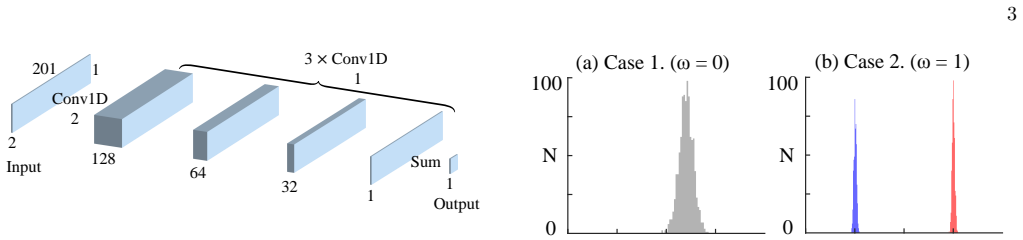
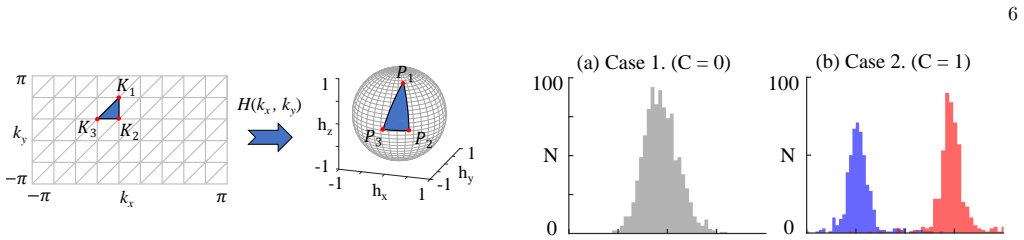
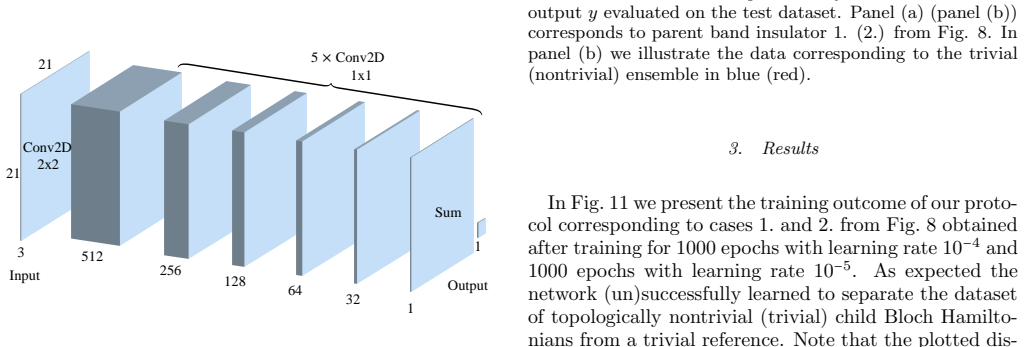
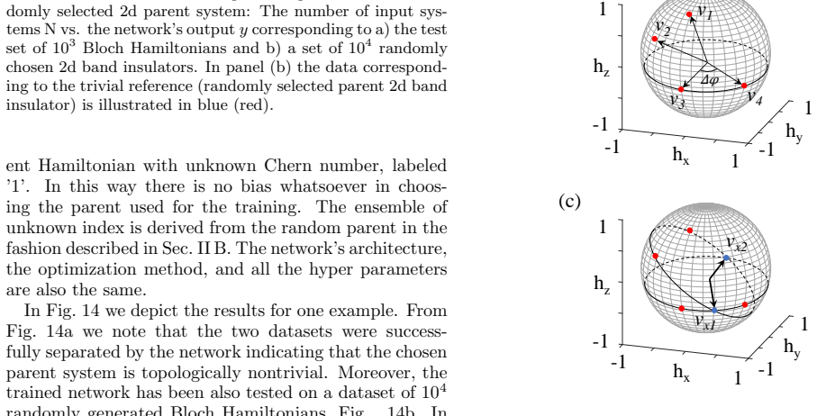
The engine is topological data augmentation: repeated random local rotations of a discretized Bloch Hamiltonian, filtered by an analytic continuity criterion so every allowed deformation is guaranteed to preserve the topological equivalence class. Discretized Hamiltonians are uniquely interpolated to continuous ones on a triangular grid; in two dimensions the allowed rotations are precisely those that keep every affected spherical triangle on the smaller hemisphere, with the acute-angled triangle check from Appendix B preventing area discontinuities. The classifier is a fully convolutional network with a summation layer, designed so the output must be a sum over local translationally invariant quantities, exactly the form of winding number and Chern number as integrals of local curvature. Learning by confusion supplies the unsupervised signal: when the network cannot separate two ensembles, achieving roughly 50% accuracy, the parent objects are topologically equivalent.
What would settle it
Take a two-dimensional parent with known Chern number, generate many children using the protocol's allowed deformations, and compute the Chern number of each child directly from the discretized Berry curvature; finding any child with a Chern number different from the parent would falsify the continuity criterion. The same check in one dimension compares winding numbers before and after each allowed rotation.
Extended reading notes
Core claim
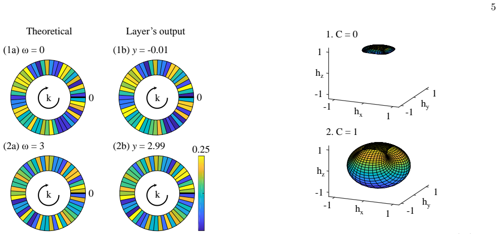
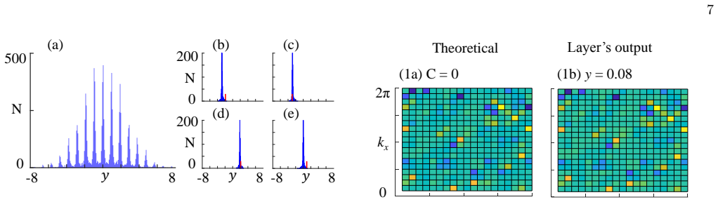
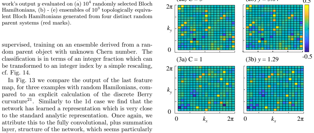
The central claim is that topological classification can be learned from unlabeled data alone, as long as one can generate topology-preserving deformations. Given a trivial reference ensemble labeled 0 and an ensemble built from a parent whose index is unknown, a convolutional network trained with learning by confusion separates the two only if the parent is nontrivial; the network's real-valued output then assigns every Bloch Hamiltonian an integer (or integer fraction) label matching its true topological index. The paper further establishes that using the augmentation in the classification step, by classifying an ensemble of topologically equivalent children of the same object, removes single-sample errors, so accuracy can be made arbitrarily close to 100% even outside the training regime. The authors verify that the learned feature maps effectively reproduce the discrete derivative of the angle in one dimension and the discretized Berry curvature in two dimensions.
Load-bearing premise
The whole protocol depends on the Appendix B continuity criterion being a correct guarantee that no allowed deformation changes the topological class of an interpolated Hamiltonian; if an allowed deformation actually crosses a class boundary, the dummy labels are wrong and everything downstream fails.
Editorial extensions
If this is right
- A network trained only on ensembles labeled 0 and 1 assigns close-to-integer outputs to arbitrary Bloch Hamiltonians, so it effectively computes winding numbers or Chern numbers over the integers and not just on the training pair.
- Classifying the full ensemble of topologically equivalent children, instead of a single sample, reaches accuracy arbitrarily close to 100% even when the individual sample output is wrong or uncertain.
- A random parent with unknown index can play the nontrivial role in training; the network then outputs labels in units of that parent's index, an integer fraction, which a trivial reference pins down to the true integer.
- The method bypasses any closed-form expression for the index, relying only on a continuity formalism for generating deformed ensembles, which opens the protocol to phases without known index formulas.
Reading between the lines
- A testable extension is to apply the same deformation-and-confusion recipe to symmetry-indicator or many-body invariants that do not yet have an efficient closed-form calculator; the protocol only needs a reliable continuity rule for the deformation.
- By extension, because the network learns to reproduce the local integrand of the index, the method could serve as a discovery tool for unknown local formulas for topological invariants in new symmetry classes.
- The need for a known trivial reference plus an unknown parent means the protocol measures the parent's index only up to an integer factor; it is fully unsupervised in the label sense but still assumes an anchor object with zero index exists and is identifiable.
- The ensemble-classification step is where the method's robustness comes from, suggesting that in future applications the cost of generating children should be weighed against the benefit of near-certain labels rather than trying to perfect single-sample outputs.
Signed reviews
Editorial analysis
A structured set of objections, weighed in public.
Referee Report
Summary. The paper proposes an unsupervised deep learning protocol for classifying topological phases. The central idea is to generate, from a small number of 'parent' Hamiltonians, large ensembles of 'children' via random topology-preserving deformations; these children are assigned dummy labels and used to train a convolutional neural network to distinguish a trivial reference ensemble from a nontrivial one, following the 'learning by confusion' scheme. The method is demonstrated for two-band insulators in 1D (winding number, class AIII) and 2D (Chern number, class A). The authors show that the trained network outputs near-integer values for random Hamiltonians, that ensembles of children of a given parent cluster at a single integer, and that using the augmentation also at the classification step can in principle yield accuracy arbitrarily close to 100% even for indices outside the training regime.
Significance. The protocol is conceptually novel: it removes the need for an auxiliary calculator of the topological index, which is the key bottleneck in earlier supervised approaches (Refs. 20 and 21). The network architecture is well matched to the problem, and the authors convincingly demonstrate that the network's last-layer output resembles the discrete Berry curvature or angle derivative. The numerical demonstrations in 1D are clean and support the central mechanism; the 2D results, while less sharp, show the expected qualitative behavior. The idea of using augmented ensembles at test time to improve classification is a valuable practical contribution. However, the correctness of the 2D protocol rests entirely on the continuity criterion of Appendix B, which is not rigorously established; this is the main obstacle to full confidence in the paper's headline claim.
major comments (2)
- [Appendix B / Sec. II.B.1] The continuity criterion that gates all 2D deformations is not rigorously defined. In Eq. (B1), the vector v_x is the intersection of the equatorial plane (through v_1 and v_2) with the circle of constant azimuthal angle θ_3, so v_x lies on the great circle through v_1 and v_2. The spherical triangle (v_1, v_2, v_x) is then degenerate, and the condition that it be 'acute' is ambiguous: the paper does not specify whether this refers to the Euclidean triangle in the plane of the great circle or to a limiting spherical triangle, nor does it define the limiting angles. Because this criterion is the only mechanism ensuring that an allowed rotation preserves the Chern number, any mislabeled child would contaminate both training and classification ensembles and would cap the achievable accuracy below 100%. I therefore request a precise definition of the degenerate case and a proof that all allowed rotations yield a globally continuous interpolated Hamiltonian, or, failing that, a numerical validation computing Chern numbers before and after a large sample of allowed rotations.
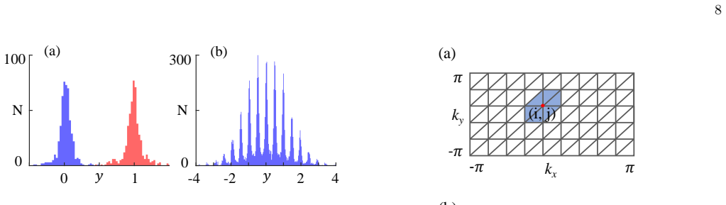
- [Sec. II.B.3 / Abstract] The claim of 'accuracy arbitrarily close to 100%' is not supported by the reported statistics. The histograms in Figs. 11 and 12 show single runs without error bars or confidence intervals, and the 'arbitrarily close' statement is an extrapolation from finite ensemble sampling rather than a demonstrated bound. Moreover, the paper does not specify a decision rule for converting the ensemble output distribution into a definite index (e.g., how many children are needed and how a peak is selected); without such a rule, the claim is not quantitatively falsifiable. In addition, if the continuity criterion of Appendix B is not guaranteed, even a small fraction of mislabeled children would prevent the accuracy from approaching 100%. The authors should provide either a probabilistic bound or a clear statistical protocol with repeated-seed experiments.
minor comments (5)
- [Sec. II.B.2] There are several typographical errors, including 'fucnctions' in the description of the 2D network and 'dervived' in Appendix A; a careful proofreading pass would improve the manuscript.
- [Appendix B] The spherical coordinate conventions used in Eq. (B1) are not stated explicitly: the text refers to 'azimuthal angle' and 'polar angle' but does not define the ranges or the relation of θ and φ to the vector components, making the derivation hard to reproduce.
- [Sec. II.A.4 / Sec. III] The necessity of a known trivial reference Hamiltonian is acknowledged only in passing ('We assume that we can always find a trivial ’0’ reference' and a similar remark in Sec. II.A.4). This is an external input that limits the universality claimed in Sec. III; it should be discussed more prominently as a limitation.
- [Figs. 4, 5, 11, 12] The histograms are presented without error bars or multiple training seeds; reporting the mean and standard deviation over several independent training runs would make the quantitative claims (especially the 98% accuracy in Fig. 11b) more robust.
- [Appendix A / Fig. 14] The inference from half-integer output peaks to an integer Chern number (C = 2) is not explained; the text says the classification is 'in terms of an integer fraction' but does not give the rescaling rule. A sentence clarifying this would help.
Circularity Check
No significant circularity: the protocol's training labels come from topology-preserving deformations, not from the topological index, and the central claims are empirically validated rather than forced by construction.
full rationale
The paper's claimed derivation chain is self-contained with respect to circularity. Training data are generated by explicit topology-preserving deformations: in 1D, rotations are allowed only when |θ_i − θ_{i±1} + φ| < π, a continuity condition on the interpolated angle; in 2D, Appendix B gives a spherical-triangle condition that forbids discontinuous changes in the interpolated Hamiltonian. These conditions are geometric and do not require evaluating the winding number or Chern number of the parent or children. The dummy labels '0' and '1' are assigned to entire ensembles, not to individual index values, and the network is tested against analytically computed indices only after training. Thus no fitted parameter is renamed as a prediction. The network architecture intentionally encodes the prior that a topological index is a sum/integral of local quantities, but the specific local function is learned from the augmented ensembles; this is an inductive bias, not a circular definition. The classification-step claim of accuracy arbitrarily close to 100% is a majority-vote statistical argument whose premise is that children of an object share its topological class. That premise is asserted via the deformation criteria; if the 2D criterion is not fully rigorous, the method could fail, but that is a correctness or soundness risk, not a circularity. There are no load-bearing self-citations: reference [42] (Andreasson et al. with Granath) appears only as an example in the introduction, and no uniqueness theorem or ansatz is imported from the authors' prior work to force the central result. The protocol does require a known trivial reference Hamiltonian and a formalism for topology-preserving deformations, but these are external inputs or assumptions, not circular redefinitions of the target index. Accordingly, no specific circular step can be exhibited, and the score is 0.
Assumptions & free parameters
free parameters (3)
- Momentum grid size in 1d (Nk=100)
- Momentum grid size in 2d (Nx=Ny=10)
- Number of deformations per 2d child (N=20 site rotations, M=50 global rotations)
assumptions (4)
- domain assumption The trivial reference Hamiltonian H=sigma_x is topologically trivial and can serve as class '0'.
- domain assumption The interpolation from discretized Hamiltonians to continuous ones (linear angle interpolation in 1d, spherical triangle interpolation in 2d) faithfully preserves topological equivalence.
- domain assumption The continuity criteria for deformations (Appendix B) are sufficient to keep the continuous interpolated system within the same topological equivalence class.
- domain assumption The network architecture (convolution plus summation) is capable of representing the topological index as a sum of local quantities for all Hamiltonians in the class.
Cite this review
Pith. "Pith review of Unsupervised learning using topological data augmentation." pith.science (2026). https://pith.science/paper/YKUDDV3X
@misc{pith2026190803469,
  author       = {Pith},
  title        = {Pith review of: Unsupervised learning using topological data augmentation},
  year         = {2026},
  howpublished = {\url{https://pith.science/paper/YKUDDV3X}},
  note         = {Machine review of arXiv:1908.03469}
}
read the original abstract
Unsupervised machine learning is a cornerstone of artificial intelligence as it provides algorithms capable of learning tasks, such as classification of data, without explicit human assistance. We present an unsupervised deep learning protocol for finding topological indices of quantum systems. The core of the proposed scheme is a 'topological data augmentation' procedure that uses seed objects to generate ensembles of topologically equivalent data. Such data, assigned with dummy labels, can then be used to train a neural network classifier for sorting arbitrary objects into topological equivalence classes. Our protocol is explicitly illustrated on 2-band insulators in 1d and 2d, characterized by a winding number and a Chern number respectively. By using the augmentation technique also in the classification step we can achieve accuracy arbitrarily close to 100% even for objects with indices outside the training regime.
Figures
Figures from the paper (9 more)

Reference graph
Works this paper leans on
-
[1]
Unsupervised learning using topological data augmentation
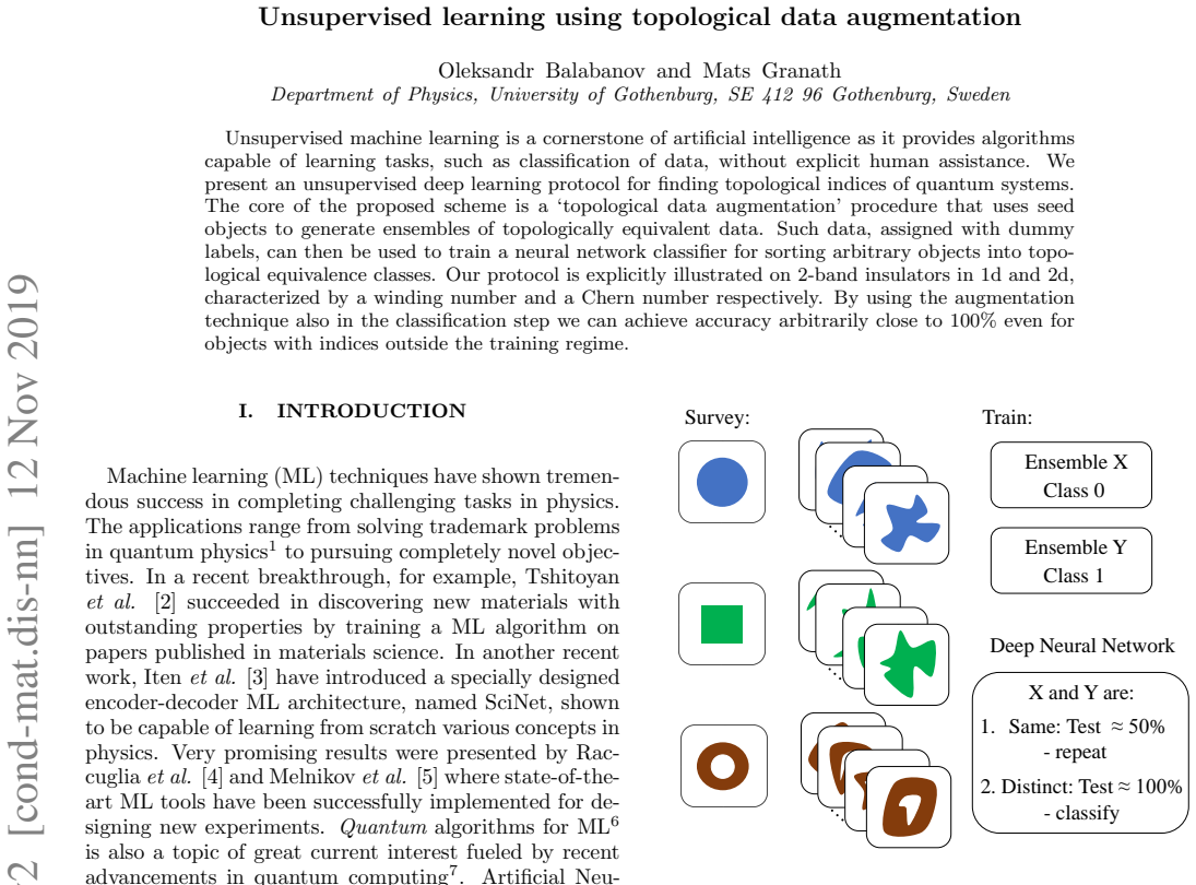
Same: Test ≈ 50% - repeat X and Y are: Ensemble Y Class 1 FIG. 1: A schematic illustration of the ‘topological data aug- mentation’ protocol for spotting topological equivalences, ap- plied to three geometric objects of different genus in 2d. By augmenting a parent object we create topologically equiva- lent ensembles and use them as input data to the ‘lea...
work page Pith review arXiv 1908
-
[2]
Distinct: Test ≈ 100% - classify
-
[3]
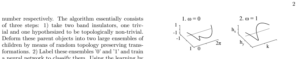
ω = 0 2. ω = 1 hx hy k FIG. 2: Examples of 1d Bloch Hamiltonians H(k) from sym- metry class AIII: 1. hx(k) = cos(k) and hy(k) = sin(k) for k ∈[0,π) and hx(k) = cos(−k) and hy(k) = sin(−k) for k ∈[π, 2π) with ω = 0; 2. hx(k) = cos(k) and hy(k) = sin(k) for k ∈[0, 2π) with ω = 1. as a function of k ∈[0, 2π). For efficiency it is practi- cal to normalize /uni2...
-
[4]
2, with known winding num- bers ω = 0 and ω = 1
Generating training data To demonstrate the algorithm we first study two par- ent systems, shown in Fig. 2, with known winding num- bers ω = 0 and ω = 1. Subsequently (Sec. II A 4) we will repeat the same analysis starting from a randomly gen- erated parent system, where ω is unknown. Although not strictly necessary it is convenient to use as baseline a re...
-
[5]
Neural network structure and training We employ the convolutional neural network depicted in Fig. 3. It consists of a 1d convolution layer of 128 filter with receptive field of size 2, which outputs 128 feature maps as lists of size 200. Following this are three 1d convolution layers of 64, 32, and 1 filters with receptive field of size 1. These layers perfor...
-
[6]
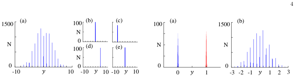
Results In Fig. 4 we plot the network’s output y evaluated on the test dataset after training for 500 epochs with learning rate 10 −4 and for 500 epochs with learning rate 10−5. The results are in agreement with our expecta- tion: The network successfully learned to distinguish the topologically nontrivial ensemble from the trivial refer- ence, Fig. 4b, b...
-
[7]
Training with unknown winding number So far we used a trivial object, labeled ’0’ and an ob- ject with known winding number ω = 1, labeled ’1’, as parents to generate the training data, with the topologi- cal index generated by the network being identical to the actual winding number for arbitrary objects. We now show that it is in fact not necessary for ...
-
[8]
A few examples, corre- sponding to random Hamiltonians, are shown in Fig
Network operation To understand why the network output label is so close to the actual winding number even for objects outside the training regime we examine the last feature map which is simply summed to give the label. A few examples, corre- sponding to random Hamiltonians, are shown in Fig. 7, where the network state is compared to a direct calcu- lati...
Show all 13 references
-
[9]
II A we here develop a scheme for finding topologically nontrivial band insulators belonging to symmetry class A in 2d
Generating training data In analogy to Sec. II A we here develop a scheme for finding topologically nontrivial band insulators belonging to symmetry class A in 2d. First we pick some parent representatives of this symmetry class, one topologically trivial (C = 0) and one nontri...
-
[10]
8: Examples of 2d band insulators: 1
C = 0 hy 1 -1hx 1 -1 -1 1 hz hy 1 -1hx 1 -1 -1 1 hz FIG. 8: Examples of 2d band insulators: 1. hx = sin(kx),hy = sin(ky), hz = 3 + cos(kx) + cos(ky) for k ∈[0, 2π) with C = 0
-
[11]
unique correspondence with continuous ones via an in- terpolation procedure schematically illustrated in Fig
hx = sin(kx), hy = sin(ky), hz = 1.5 + cos(kx) + cos(ky) for k ∈[0, 2π) with C = 1 . unique correspondence with continuous ones via an in- terpolation procedure schematically illustrated in Fig. 9. In short, we define a triangular grid in 2d momentum space and interpolate discr...
-
[12]
II A but now extended to 2d layered input as shown in Fig
2d Convolutional Network The neural network trained to classify this data is sim- ilar to that in Sec. II A but now extended to 2d layered input as shown in Fig. 10. We employ a 2d convolutional layer of 512 filters with 2 × 2 receptive field, that outputs 512 feature maps of di...
-
[13]
11 we present the training outcome of our proto- col corresponding to cases 1
Results In Fig. 11 we present the training outcome of our proto- col corresponding to cases 1. and 2. from Fig. 8 obtained after training for 1000 epochs with learning rate 10−4 and 1000 epochs with learning rate 10 −5. As expected the network (un)successfully learned to separ...
2018 arXiv
Reviewed August 14, 2026 · model on record in the stance chip above.
Discussion (0). Continue with ORCID to comment.