BoltzmaNN: Predicting effective pair potentials and equations of state using neural networks

Arash Nikoubashman; Fabian Berressem

REVIEW 3 major objections 4 minor 19 references

BoltzmaNN: Predicting effective pair potentials and equations of state using neural networks

T0 review · 3 major / 4 minor · reviewed 2026-08-14 · deepseek-v4-flash

Challenge this review Re-run · record.json Download PDF Read on arXiv ↗ Review JSON

Pith's one-line read Trained neural networks can predict equations of state and recover effective pair potentials from radial distribution functions with errors an order of magnitude below standard analytic estimates.

desk verdict Useful ML-for-soft-matter study with a real data-split leak that needs fixing before the accuracy claims can be trusted. read the letter →

arxiv 1908.02448 v2 pith:YN7BUZEU submitted 2019-08-07 cond-mat.soft cond-mat.dis-nn

Fabian Berressem , Arash Nikoubashman This is my paper · ORCID

classification cond-mat.softcond-mat.dis-nn PACS 05.20.Jj61.20.Ja64.10.+h

keywords neuralnetworksequationofstatevirialcoefficientspairpotentialsradialdistributionfunctioncoarse-grainingBoltzmanninversionmoleculardynamicssimulation

verification ladder T0 review T1 audit T2 compute T3 formal

The pith

A machine-rendered reading of the paper's core claim, the machinery that carries it, and where it could break.

The reading

This paper tries to show that a single trained neural network can replace two standard statistical-mechanics approximations: the low-density virial estimate for equations of state, and Boltzmann inversion for recovering pair potentials from structure. For the forward direction, a U-Net is trained to turn a pair potential into density-independent virial coefficients B2 through B5, and the pressure follows from the virial expansion; on held-out potentials this reaches a mean relative pressure error around 0.11, where the analytic second-virial estimate is off by roughly an order of magnitude. For the inverse direction, a convolutional network maps a measured radial distribution function to the underlying potential, and including force information in the training loss cuts the typical potential error from about 0.5 kBT under Boltzmann inversion to about 0.03 kBT while making the output smoother and more transferable across densities. If correct, this offers a fast, one-shot route to effective potentials for coarse-graining and inverse design, without iterative simulation loops.

What carries the argument

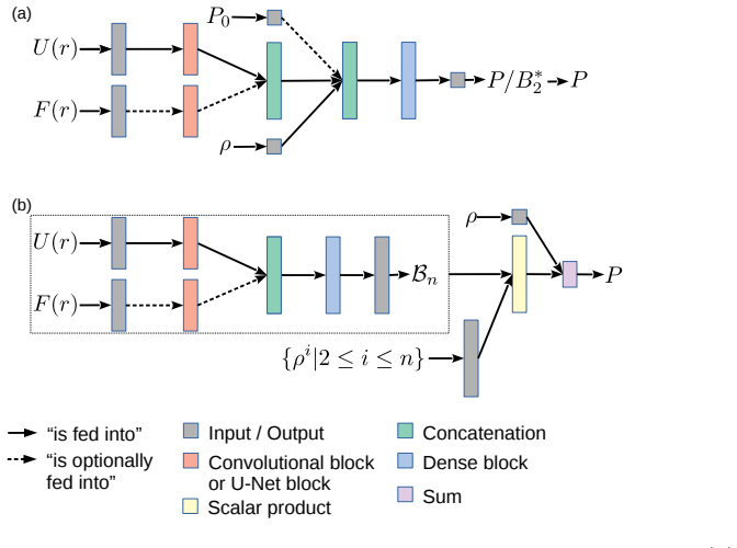
The load-bearing construction is the virial-coefficient layer: instead of mapping U(r) directly to pressure, the network outputs density-independent coefficients B2 through B5, and fixed, parameter-free layers compute βP = ρ + $B2ρ^{2}$ + $B3ρ^{3}$ + $B4ρ^{4}$ + $B5ρ^{5}$. This forces the density dependence to come from the virial expansion rather than from the network, which is why the model extrapolates better than a direct U-to-P map. For the inverse problem, the crucial mechanism is a loss augmented with force information: the network trains not only on U(r) values but on their finite-difference derivatives, through terms like the discretized Laplacian and difference-correlation losses, so the predicted potential is constrained to vary smoothly. Input clipping, capping U at 20 kBT, and, for the inverse side, using the Boltzmann estimate U0(r) as input are supporting representations that keep the network's search space bounded.

What would settle it

Take the trained pressure and potential networks and evaluate them on a held-out family of potentials that the spline generator cannot produce, for example long-ranged Yukawa or SALR potentials with a repulsive barrier, and compare pressure and potential errors to the reported values of about 0.11 mean relative error and 0.03 kBT; a substantial error increase would show the training family was not representative. A cheaper check is to re-run the benchmark including the 787 discarded simulations and see whether test errors rise.

Watch

Extended reading notes

Core claim

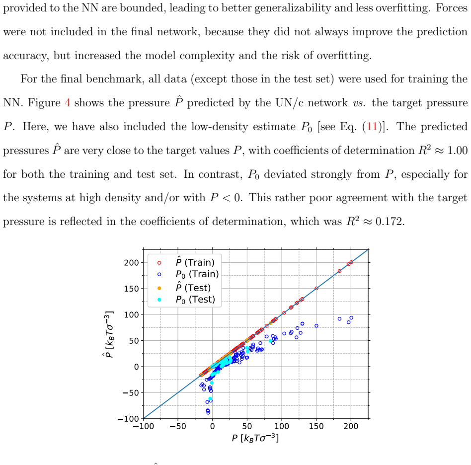
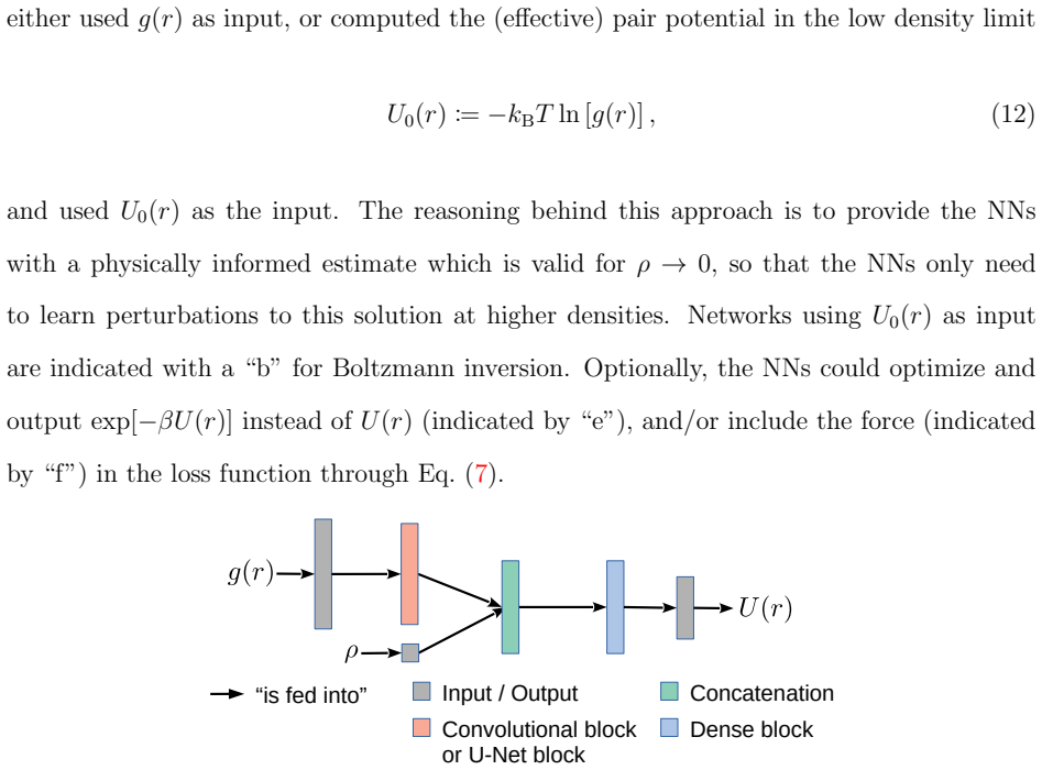
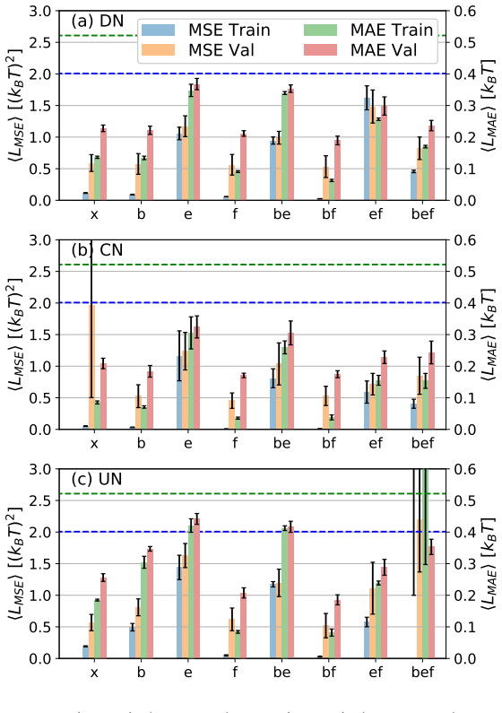
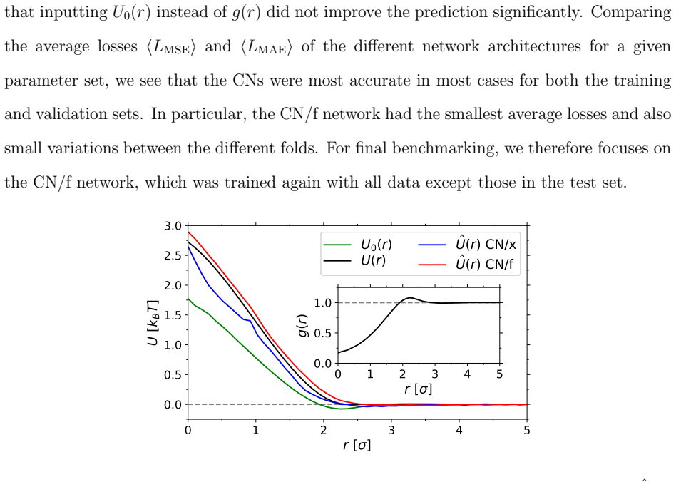
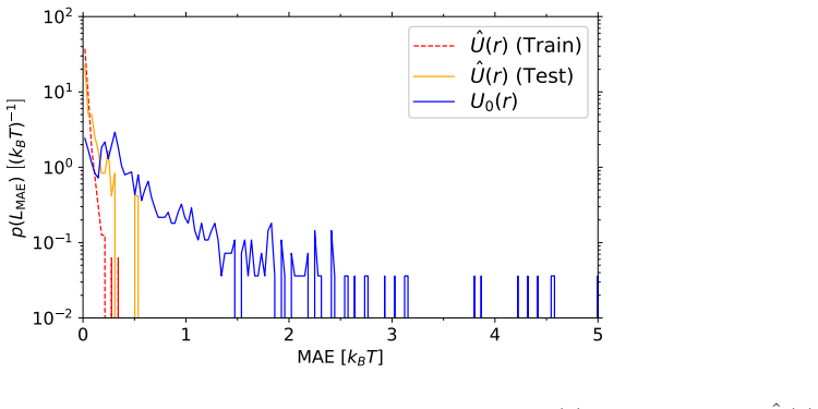
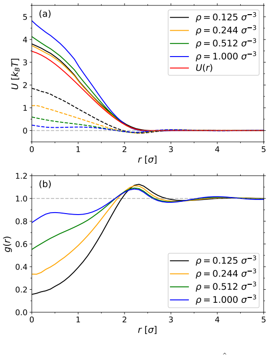
The central claim is that machine-learned maps can carry the physics that the analytic low-density limit misses. Networks that first predict the virial coefficients {B2,...,B5} from a pair potential and then form the pressure through the virial expansion reproduce simulation pressures with R²≈1.00 on both training and test data, whereas the second-virial estimate has R²≈0.172 and misses negative pressures entirely. On the inverse problem, a convolutional network fed g(r) at a known density, with the potential derivative included in the loss, recovers U(r) with an exponential error distribution of width δ≈0.03 kBT on the test set, compared with δ≈0.5 kBT for U0 = -kBT ln g(r); the recovered potentials reproduce g(r) in fresh simulations and remain nearly independent of the density at which g(r) was measured. The paper also shows the two networks can be chained: potentials predicted from g(r) feed into the pressure network, giving R²≈0.971 on training data and R²≈0.461 on the test set.

Load-bearing premise

The accuracy claims depend on the 657 randomly generated spline potentials that survived the simulations being representative of real isotropic pair potentials; if the discarded simulations or unseen potential shapes are systematically harder, the reported test-set errors will not carry over to applications.

Editorial extensions

If this is right

Pressure predictions from the chosen U-Net stay accurate on densities not seen in training, because the learned B2 through B5 are density-independent and only the polynomial in density is evaluated.
The inverse convolutional network gives potentials that are smoother and closer to the target than Boltzmann inversion, with the predicted potential varying little between g(r) curves measured at different densities.
Predicted potentials can serve as initial guesses for iterative refinement methods such as Iterative Boltzmann Inversion, replacing a poor U0 start and reducing the number of simulation cycles needed.
Chaining the two networks provides an end-to-end route from structure g(r) to pressure, with near-simulation accuracy on training data and correct trends on the test set.
Because pressure comes from learned virial coefficients, the approach inherits the virial expansion's limitation: it is most reliable where the series converges, and the reported accuracy applies to the densities and potential shapes in the training family.

Reading between the lines

Editorial extensions of the paper, not claims the author makes directly.

If the training family were expanded to include long-ranged or bounded potentials, for example screened Coulomb or cluster-forming potentials with repulsive barriers, the same two-stage architecture would plausibly extend to the soft-matter systems the introduction motivates; the current spline family has no such features, so this is an open test rather than a paper claim.
The paper's differing verdict on force information, helpful for recovering potentials but unnecessary or harmful for predicting pressure, suggests the force input matters most when the network must learn derivatives; a shared network with force inputs on both tasks could be tested against the separate designs.
Because 47% of simulations were discarded before training, a useful stress test would be to keep the discarded configurations and compare errors; if the network fails preferentially on those, the reported test-set accuracy overstates real-world robustness.
The end-to-end g(r)-to-pressure chain's drop from R²≈0.971 on training data to 0.461 on the test set hints that error accumulates through the two networks, and a combined loss trained on the full chain might close much of that gap.

Share X Bluesky LinkedIn Reddit HN

Signed reviews

No signed human review yet.

Editorial analysis

A structured set of objections, weighed in public.

Desk editor's note, referee report, and a circularity audit.

Desk Editor's Note

read the letter

Colleague —

Quick take on Berressem/Nikoubashman (arXiv:1908.02448): the paper does useful, honest work on two ML tasks — mapping pair potentials to equations of state and inverting g(r) to effective potentials — but the headline accuracy numbers are undercut by an unstated train/test split policy that likely leaks potentials between training and test. That needs to be resolved before taking the numbers at face value.

What is genuinely new here: the virial-coefficient intermediate representation (U -> B2...B5 -> P) is a clean idea and clearly helps extrapolate in density; the force-aware loss for potential inversion is a small but real improvement in smoothness and accuracy over plain Boltzmann inversion, with δ ≈ 0.03 kBT on the test set versus 0.5 kBT for U0(r). The systematic comparison of clipped vs exponential inputs and the ablation of force info is more thorough than most papers in this niche. They ship code and example scripts, which is good.

Soft spots, in order of severity.

First, the split. Section 2.2 says 657 potentials, 1678 simulations, 891 retained points, and 790/101 train/test split. It never says the split is disjoint by potential. Since each potential is simulated at up to four densities, a random point-wise split almost certainly puts the same potential in both train and test at different densities. For the EOS net the input includes U(r) and rho, so the network can memorize a training potential and merely interpolate in rho. Same for the g-to-U net. The stress-test note is right: without a potential-disjoint split, the LMRAE ≈ 0.11 and δ ≈ 0.03 numbers are not a valid test of generalization to new potentials. This is a fixable issue but it's load-bearing.

Second, the data filtering. 47% of simulations discarded, with criteria in the ESI. We only have the paper, so I can't judge whether the remaining set is representative, but the authors should quantify how many of the discarded cases are tied to specific potential shapes. If the hard cases correlate with features that matter in real soft matter, the trained nets will be optimistic.

Third, the end-to-end pipeline (g to U to P) drops to R^2=0.461 on the test set. The authors are honest about it, but it means the practical usefulness for coarse-graining is still limited.

Fourth, no quantitative comparison with IBI or RMC. The conclusion mentions they expect lower accuracy than iterative methods, but a direct benchmark on the same test potentials would make the 'fast initial estimate' claim much stronger.

Who is it for: anyone working on ML-based coarse-graining or inverse design in soft matter. The force-aware loss idea and the virial-coefficient output representation are worth discussing. I'd bring it to a reading group as a good case study in data-split pitfalls.

Recommendation: it deserves serious peer review, but only after the authors clarify—or redo—the train/test split by potential and report how many potentials actually survive. If the split was point-wise, the central generalization claims need to be recomputed. As is, I would not trust the reported test errors.

Referee Report

3 major / 4 minor

Summary. The manuscript introduces neural-network surrogates for two complementary tasks in soft-matter physics: predicting the equation of state from an isotropic pair potential U(r) via learned virial coefficients, and recovering (effective) pair potentials from radial distribution functions g(r). Training data come from 1678 MD simulations on 657 randomly generated spline potentials at four densities, reduced to 891 usable data points after discarding non-equilibrated or heterogeneous runs. The authors compare dense, convolutional, and U-Net architectures, input representations (U, clipped U, exp[-beta U]), and auxiliary inputs such as forces and low-density pressure estimates. They report that a U-Net with clipped potentials predicting B2 through B5 gives near-unity R^2 for pressure, and that a convolutional network with force information in the loss recovers potentials with MAE width delta about 0.03 kBT, far better than Boltzmann inversion. A composite g-to-U-to-P pipeline is also tested, with R^2 about 0.46 on the test set.

Significance. If the reported accuracy and transferability hold, the paper makes a useful practical contribution: it provides fast, differentiable surrogates for the virial equation of state and for inverse coarse-graining, with code released, physically motivated output representations, and a genuine end-to-end out-of-sample check (g to U to P). The systematic ablation of input representations, force information, and loss terms is a strength, and the explicit comparison against the low-density analytic second-virial estimate places the gains in context. The main uncertainty is not methodological novelty but whether the benchmark is trustworthy under a properly disjoint train/test split; the potential-level leakage concern, if real, would invalidate the quantitative claims in Sections 3.1 and 3.2.

major comments (3)

[Sec. 2.2, data split] The paper does not state whether the 790/101 train/test split and the 4-fold cross-validation used for architecture selection are disjoint at the level of pair potentials. Because each potential is simulated at up to four densities, a random split of the 891 data points would place different densities of the same U(r) in both training and test sets. For the U(r)-to-P networks this would let the network interpolate in density for potentials it has already seen; for the g(r)-to-U networks the target potential itself would be memorized. Since the central generalization claims in Sections 3.1 and 3.2 depend on unseen potentials, the authors must either state explicitly that no potential appears in both training and test partitions, or redo the split and all reported benchmarks (including the cross-validation in Sec. 2.1) with potential-disjoint folds.
[Sec. 2.2, data filtering] About 47% of the 1678 simulations were discarded because they did not reach equilibrium or formed heterogeneous structures, with the exclusion criteria deferred to the ESI. This filtering is not a neutral preprocessing step: it removes exactly the states where the underlying physics is most complex, so the training distribution may be systematically easier than the distribution of real soft-matter systems to which the networks are advertised. The authors should quantify the excluded cases (e.g., by density, potential shape, and pressure range) and demonstrate that the reported held-out errors are not an artifact of this screening; without this, the transferability claims in the abstract and conclusions are not supported.
[Sec. 3.2, Fig. 11] The composite pipeline from g(r) through the predicted potential to pressure achieves R^2=0.461 on the test set, and this is the only end-to-end benchmark that exercises both networks together. The paper should report this limitation prominently in the abstract or conclusions and explain the outlier at P approximately 80 kBT/sigma^3: is it within the training density/potential range, and does it correspond to a regime where the discarded simulations would have been relevant? As written, the central 'much more accurate' claim is based on the direct U-to-P task, but a reader applying the method to experimental g(r) will face the composite accuracy, so the discrepancy matters for the stated use case.

minor comments (4)

[Sec. 3.2, Fig. 10 caption] In the caption, the LMSE value for case (b) is printed as 5.7 x 10^3, which is likely a typo for 5.7 x 10^-3; please correct it, as the comparison with the other cases suggests the exponent is wrong.
[References] Reference 18 lists 'J. Chem. Phys. 2018, DETC2018, 241706'; the volume and article identifier appear inconsistent with the journal's format and should be checked.
[Sec. 2.2, Fig. 1] The inset of Fig. 7 and the axis labels in Fig. 1 would benefit from stating that r is in units of sigma explicitly on the axes, rather than only in the text, for clarity.
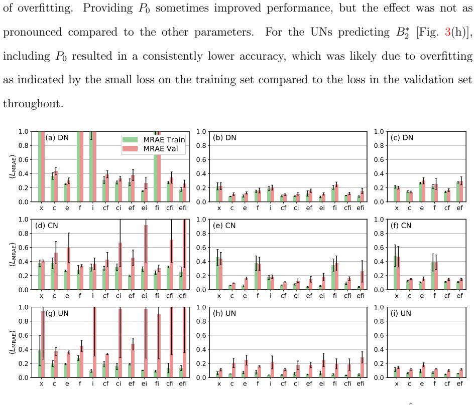
[Sec. 3.1, Fig. 4] The text says the training-set LMRAE for UN/c is about 0.06 and the test-set about 0.11, but Fig. 3 shows only train/validation values; stating the test value in the figure caption or in the text where the network is chosen would help the reader connect the figures.

Circularity Check

0 steps flagged · score 0.0 of 10

No significant circularity: the networks are benchmarked on held-out MD data, and the predicted quantities are not defined in terms of the targets.

full rationale

The paper's central claims are supported by out-of-sample evaluation: neural networks are trained on MD simulation data and tested on held-out simulations, with no adjustable parameters re-entering the definition of the target quantities. For the EOS task, the network maps U(r) to virial coefficients or directly to pressure, and the final pressure is computed through an explicit virial expansion using density-independent learned coefficients; the analytic low-density B2 estimate is used only as a baseline. For the potential-inversion task, the network maps g(r) or the Boltzmann-inversion estimate U0(r) to U(r), with the loss evaluated against the target U(r), and the composite g-to-U-to-P test provides an additional independent check. None of the reported outputs (B2*, Bn, or U-hat) is defined in terms of the quantities it is supposed to predict, and no fitted parameter is renamed as a prediction. Self-citations are confined to a software repository link and a contextual coarse-graining reference; neither is load-bearing. Any potential concern about whether the train/test split was disjoint at the level of potentials would be a data-leakage or generalization issue, not a circularity of derivation. Under the evidentiary standard requiring a specific reduction of a prediction to its inputs, no circular step is present.

Assumptions & free parameters 7 free parameters · 5 assumptions · 0 invented entities

The paper introduces no new physical entities. It rests on standard statistical mechanics (virial expansion, Henderson uniqueness, Boltzmann inversion) and on empirical machine-learning assumptions that the generated spline potentials and the surviving MD simulations are representative and that the networks generalize. The hand-chosen clipping and loss weights are enumerated above.

free parameters (7)

Ucut potential clipping threshold = 20 kBT
Used to cap input/output potentials; the authors state the choice is 'somewhat arbitrary' but tests show little effect as long as it separates soft and hard potentials (Sec. 3.1).
Loss weight alpha_Delta = 2
Weight for the discretized Laplace term in the potential-prediction loss, Eq. (5).
Loss weight alpha for Lk terms = 1
Optional multiplier for distance-correlation loss terms, Eq. (5).
Number of virial coefficients = 5 (B2 to B5)
The pressure network predicts five density-independent virial coefficients; higher-order or density-dependent terms are not included.
Simulation densities = 0.125, 0.244, 0.512, 1.0 sigma^-3
Four densities chosen to span gas and liquid regimes; density dependence is only sampled at these points.
Downsampled potential grid = 50 points
Potentials and g(r) are represented on a 50-point grid in [0,5 sigma], which limits the resolution of the inputs and outputs.
Spline potential generation range = n in [6,10], magnitudes in [0,15 kBT], spline degree in [2,5]
Random generation parameters that determine the family of potentials in the training set.

assumptions (5)

domain assumption Virial expansion of the pressure converges with a small number of density-independent coefficients for the potentials and densities studied.
The pressure network explicitly uses beta P = rho + sum_{i=2}^{5} B_i rho^i (Strategy 3, Sec. 3.1).
domain assumption Henderson's uniqueness theorem: a given g(r) determines the pair potential up to an additive constant at a fixed density.
Justifies the inverse problem of recovering U(r) from g(r); cited as ref 37 but not proved.
standard math The Boltzmann inversion U0 = -kBT ln g(r) is the correct low-density limit estimate, used as an input representation and baseline.
Eq. (12), Sec. 3.2.
domain assumption Canonical NVT sampling with a Langevin thermostat and Velocity-Verlet integration produces equilibrium P and g(r) for the tabulated potentials.
Sec. 2.2 data generation.
domain assumption The neural networks have sufficient capacity and the optimizer finds parameters that generalize from the training distribution.
Standard supervised learning assumption; no formal guarantees are given.

how reviews work

0 comments

Cite this review

Pith. "Pith review of BoltzmaNN: Predicting effective pair potentials and equations of state using neural networks." pith.science (2026). https://pith.science/paper/YN7BUZEU

@misc{pith2026190802448,
  author       = {Pith},
  title        = {Pith review of: BoltzmaNN: Predicting effective pair potentials and equations of state using neural networks},
  year         = {2026},
  howpublished = {\url{https://pith.science/paper/YN7BUZEU}},
  note         = {Machine review of arXiv:1908.02448}
}

abstract

Neural networks (NNs) are employed to predict equations of state from a given isotropic pair potential using the virial expansion of the pressure. The NNs are trained with data from molecular dynamics simulations of monoatomic gases and liquids, sampled in the $NVT$ ensemble at various densities. We find that the NNs provide much more accurate results compared to the analytic low-density limit estimate of the second virial coefficient. Further, we design and train NNs for computing (effective) pair potentials from radial pair distribution functions, $g(r)$, a task which is often performed for inverse design and coarse-graining. Providing the NNs with additional information on the forces greatly improves the accuracy of the predictions, since more correlations are taken into account; the predicted potentials become smoother, are significantly closer to the target potentials, and are more transferable as a result.

Figures

Figures reproduced from arXiv: 1908.02448 by the authors.

**Figure 1.** (a) Three selected pair potentials U(r) used in this work, and (b) corresponding radial pair distribution functions, g(r), recorded at particle number density ρ = 0.125 σ −3 . (c) g(r) for UI at three investigated values of ρ, as indicated. 8 [PITH_FULL_IMAGE:figures/full_fig_p008_1.png] view at source ↗

**Figure 2.** Schematic representation of the NNs used for computing the pressure [PITH_FULL_IMAGE:figures/full_fig_p010_2.png] view at source ↗

**Figure 3.** Mean relative absolute error hLMRAEi between predicted pressures Pˆ and target pressures P for different NN architectures and options. The panels are ordered from top to bottom as DN, CN and UN and from left to right as mapping to P, mapping to B∗ 2 and mapping to Bn. Based on the comparison shown in [PITH_FULL_IMAGE:figures/full_fig_p013_3.png] view at source ↗

Figures from the paper (8 more)

**Figure 4.** Figure 4: Predicted pressure Pˆ from UN/c (red and orange symbols) and P0 estimated from Eq. (11) (blue and cyan symbols) vs. the target pressure P. Open and filled symbols show results from the training and test set, respectively. 3.2 Potential prediction from pair distribution…

**Figure 5.** Figure 5: Schematic representation of the NNs used for predicting (effective) pair potentials [PITH_FULL_IMAGE:figures/full_fig_p015_5.png]

**Figure 6.** Figure 6: Comparison of hLMSEi (left axis) and hLMAEi (right axis) between the predicted, Uˆ(r), and target pair potential, U(r), for (a) DNs, (B) CNs, and (c) UNs with different options (see [PITH_FULL_IMAGE:figures/full_fig_p017_6.png]

**Figure 7.** Figure 7: Selected target pair potential U(r) from the validation set and predictions Uˆ(r) from CN/x and CN/f. The estimated potential U0(r) is also shown for comparison. The inset shows the corresponding radial distribution function g(r) at the employed density ρ = 0.125 σ −3 …

**Figure 8.** Figure 8: Probability density function of LMAE between target U(r) and predicted Uˆ(r) using CN/f, and between U(r) and U0(r). Given that g(r) can vary significantly for the same U(r) at different particle number densities ρ, it is important to check whether Uˆ(r) remains indepe…

**Figure 9.** Figure 9: (a) Target potential U(r) and predicted potentials Uˆ(r) from CN/f at four different particle number densities ρ, as indicated. The dashed lines show U0(r) at the same densities. (b) Radial pair distribution functions g(r) from simulations with U(r) at various ρ, as i…

**Figure 10.** Figure 10: Comparison between radial pair distribution functions [PITH_FULL_IMAGE:figures/full_fig_p022_10.png]

**Figure 11.** Figure 11: Predicted pressure Pˆ from UN/c (red and orange symbols) and P0 estimated from Eq. (11) (blue and cyan symbols) vs. the target pressure, P, using the potentials Uˆ(r) and U0(r), respectively. Open and filled symbols show results from the training and testing set, resp…

Discussion (0). Continue with ORCID to comment.

Reference graph

Works this paper leans on

19 extracted references · 19 canonical work pages

[1]

G.; Frenkel, D

(1) Noro, M. G.; Frenkel, D. Extended corresponding-states behavior for particles with variable range attractions. J. Chem. Phys. 2000, 113, 2941–2944. (2) Lu, P. J.; Zaccarelli, E.; Ciulla, F.; Schoﬁeld, A. B.; Sciortino, F.; Weitz, D. A. Gelation of particles with short-range attraction. Nature 2008, 453,

work page 2000
[66]

(22) Schmidt, J.; Marques, M. R. G.; Botti, S.; Marques, M. A. L. Recent advances and applications of machine learning in solid-state materials science. npj Comput. Mater. 2019, 5,

work page 2019
[83]

L.; Pusztai, L

26 (23) McGreevy, R. L.; Pusztai, L. Reverse Monte Carlo Simulation: A New Technique for the Determination of Disordered Structures. Mol. Simul. 1988, 1, 359–367. (24) Keen, D.; McGreevy, R. Structural modelling of glasses using reverse Monte Carlo simulation. Nature 1990, 344,

work page 1988
[106]

Machine- learning-assisted discovery of polymers with high thermal conductivity using a molec- ular design algorithm

(21) Wu, S.; Kondo, Y.; Kakimoto, M.-a.; Yang, B.; Yamada, H.; Kuwajima, I.; Lam- bard, G.; Hongo, K.; Xu, Y.; Shiomi, J.; Schick, C.; Morikawa, J.; Yoshida, R. Machine- learning-assisted discovery of polymers with high thermal conductivity using a molec- ular design algorithm. npj Comput. Mater. 2019, 5,

work page 2019
[197]

Comparative atomistic and coarse-grained study of water: What do we lose by coarse-graining? Eur

(38) Wang, H.; Junghans, C.; Kremer, K. Comparative atomistic and coarse-grained study of water: What do we lose by coarse-graining? Eur. Phys. J. E 2009, 28, 221–229. (39) Das, A.; Andersen, H. C. The multiscale coarse-graining method. V. Isothermal-isobaric ensemble. J. Chem. Phys. 2010, 132, 164106. (40) Bereau, T.; Rudzinski, J. F. Accurate Structure-...

work page 2009
[347]

Coarsegraining in polymer simulation: From the atomistic to the mesoscopic scale and back

(31) M¨ uller-Plathe, F. Coarsegraining in polymer simulation: From the atomistic to the mesoscopic scale and back. ChemPhysChem 2002, 3,

work page 2002
[423]

P.; Laaksonen, A

(25) Lyubartsev, A. P.; Laaksonen, A. Calculation of eﬀective interaction potentials from radial distribution functions: A reverse Monte Carlo approach. Phys. Rev. E 1995, 52,

work page 1995
[499]

Accurate eﬀective pair potentials for polymer solutions

24 (3) Bolhuis, P.; Louis, A.; Hansen, J.; Meijer, E. Accurate eﬀective pair potentials for polymer solutions. J. Chem. Phys. 2001, 114, 4296–4311. (4) Likos, C. N. Eﬀective interactions in soft condensed matter physics. Phys. Rep. 2001, 348, 267–439. (5) Sciortino, F.; Mossa, S.; Zaccarelli, E.; Tartaglia, P. Equilibrium cluster phases and low- density a...

work page 2001

Show all 19 references

[539]

Perspective: Machine learning potentials for atomistic simulations

(15) Behler, J. Perspective: Machine learning potentials for atomistic simulations. J. Chem. Phys. 2016, 145, 170901. (16) Audus, D. J.; de Pablo, J. J. Polymer informatics: Opportunities and challenges. ACS Macro Lett. 2017, 6,

2016
[754]

Mapping atomistic simulations to mesoscopic models: A 27 systematic coarse-graining procedure for vinyl polymer chains

(32) Milano, G.; M¨ uller-Plathe, F. Mapping atomistic simulations to mesoscopic models: A 27 systematic coarse-graining procedure for vinyl polymer chains. J. Phys. Chem. B 2005, 109, 18609. (33) Bayramoglu, B.; Faller, R. Coarse-grained modeling of polystyrene in various env...

2005
[1078]

(17) Ferguson, A. L. Machine learning and data science in soft materials engineering. J. Phys.: Condens. Matter 2017, 30, 043002. (18) Bereau, T.; DiStasio Jr., R. A.; Tkatchenko, A.; von Lilienfeld, A. O. Non-covalent interactions across organic and biological subsets of chem...

2017
[1624]

C.; Stillinger, F

(27) Rechtsman, M. C.; Stillinger, F. H.; Torquato, S. Optimized interactions for targeted self-assembly: application to a honeycomb lattice. Phys. Rev. Lett 2005, 95, 228301. (28) Reatto, K.; Levesque, D.; Weiss, J. J. Iterative predictor-corrector method for extrac- tion of ...

2005
[2015]

(47) Abadi, M.; Agarwal, A.; Barham, P.; Brevdo, E.; Chen, Z.; Citro, C.; Corrado, G

Cham, 2015; pp 234–241. (47) Abadi, M.; Agarwal, A.; Barham, P.; Brevdo, E.; Chen, Z.; Citro, C.; Corrado, G. S.; Davis, A.; Dean, J.; Devin, M.; Ghemawat, S.; Goodfellow, I.; Harp, A.; Irving, G.; Isard, M.; Jia, Y.; Jozefowicz, R.; Kaiser, L.; Kudlur, M.; Levenberg, J.; Man´...

2015
[3451]

N.; Dobnikar, J.; Nikoubashman, A

(29) M¨ uller, K.; Osterman, N.; Babiˇ c,; Likos, C. N.; Dobnikar, J.; Nikoubashman, A. Pattern formation and coarse-graining in two-dimensional colloids driven by multiaxial magnetic ﬁelds. Langmuir 2014, 30,

2014
[3730]

Deriving eﬀective mesoscale potentials from atomistic simulations

(26) Reith, D.; P¨ utz, M.; M¨ uller-Plathe, F. Deriving eﬀective mesoscale potentials from atomistic simulations. J. Comput. Chem. 2003, 24,

2003
[5088]

Thermodynamics of hydrophobic amino acids in solution: A combined experimentalcomputational study

(30) Song, L.; Yang, L.; Meng, J.; Yang, S. Thermodynamics of hydrophobic amino acids in solution: A combined experimentalcomputational study. J. Phys. Chem. Lett. 2017, 8,

2017
[6702]

R.; Hannon, A

25 (14) Gadelrab, K. R.; Hannon, A. F.; Ross, C. A.; Alexander-Katz, A. Inverting the design path for self-assembled block copolymers. Mol. Syst. Des. Eng. 2017, 2,

2017
[9187]

(35) Rosenberger, D.; Hanke, M.; van der Vegt, N. F. A. Comparison of iterative inversecoarse-graining methods. Eur. Phys. J. Special Topics 2016, 225, 1323–1345. (36) Shell, M. S. The relative entropy is fundamental to multiscale and inverse thermody- namic problems. J. Chem....

2016
[9205]

(34) Louis, A. A. Beware of density dependent pair potentials. J. Phys.: Condens. Matter 2002, 14,

2002

Pith tools

Reviewed August 14, 2026 · model on record in the stance chip above.

[1] [1]

G.; Frenkel, D

(1) Noro, M. G.; Frenkel, D. Extended corresponding-states behavior for particles with variable range attractions. J. Chem. Phys. 2000, 113, 2941–2944. (2) Lu, P. J.; Zaccarelli, E.; Ciulla, F.; Schoﬁeld, A. B.; Sciortino, F.; Weitz, D. A. Gelation of particles with short-range attraction. Nature 2008, 453,

work page 2000

[2] [66]

(22) Schmidt, J.; Marques, M. R. G.; Botti, S.; Marques, M. A. L. Recent advances and applications of machine learning in solid-state materials science. npj Comput. Mater. 2019, 5,

work page 2019

[3] [83]

L.; Pusztai, L

26 (23) McGreevy, R. L.; Pusztai, L. Reverse Monte Carlo Simulation: A New Technique for the Determination of Disordered Structures. Mol. Simul. 1988, 1, 359–367. (24) Keen, D.; McGreevy, R. Structural modelling of glasses using reverse Monte Carlo simulation. Nature 1990, 344,

work page 1988

[4] [106]

Machine- learning-assisted discovery of polymers with high thermal conductivity using a molec- ular design algorithm

(21) Wu, S.; Kondo, Y.; Kakimoto, M.-a.; Yang, B.; Yamada, H.; Kuwajima, I.; Lam- bard, G.; Hongo, K.; Xu, Y.; Shiomi, J.; Schick, C.; Morikawa, J.; Yoshida, R. Machine- learning-assisted discovery of polymers with high thermal conductivity using a molec- ular design algorithm. npj Comput. Mater. 2019, 5,

work page 2019

[5] [197]

Comparative atomistic and coarse-grained study of water: What do we lose by coarse-graining? Eur

(38) Wang, H.; Junghans, C.; Kremer, K. Comparative atomistic and coarse-grained study of water: What do we lose by coarse-graining? Eur. Phys. J. E 2009, 28, 221–229. (39) Das, A.; Andersen, H. C. The multiscale coarse-graining method. V. Isothermal-isobaric ensemble. J. Chem. Phys. 2010, 132, 164106. (40) Bereau, T.; Rudzinski, J. F. Accurate Structure-...

work page 2009

[6] [347]

Coarsegraining in polymer simulation: From the atomistic to the mesoscopic scale and back

(31) M¨ uller-Plathe, F. Coarsegraining in polymer simulation: From the atomistic to the mesoscopic scale and back. ChemPhysChem 2002, 3,

work page 2002

[7] [423]

P.; Laaksonen, A

(25) Lyubartsev, A. P.; Laaksonen, A. Calculation of eﬀective interaction potentials from radial distribution functions: A reverse Monte Carlo approach. Phys. Rev. E 1995, 52,

work page 1995

[8] [499]

Accurate eﬀective pair potentials for polymer solutions

24 (3) Bolhuis, P.; Louis, A.; Hansen, J.; Meijer, E. Accurate eﬀective pair potentials for polymer solutions. J. Chem. Phys. 2001, 114, 4296–4311. (4) Likos, C. N. Eﬀective interactions in soft condensed matter physics. Phys. Rep. 2001, 348, 267–439. (5) Sciortino, F.; Mossa, S.; Zaccarelli, E.; Tartaglia, P. Equilibrium cluster phases and low- density a...

work page 2001