REVIEW 3 major objections 6 minor 61 references
A Visibility-based 21 cm Bispectrum Estimator for Radio-interferometric Data
T0 review · 3 major / 6 minor · reviewed 2026-08-07 · deepseek-v4-flash
Pith's one-line read A visibility-based, FFT-accelerated estimator recovers the binned multi-frequency angular bispectrum and the 3D 21 cm bispectrum from radio-interferometric data, validated on simulated MWA observations with deviations below 20 percent.
desk verdict A solid, self-consistent extension of the visibility-based bispectrum estimator to multi-frequency and 3D, but the 3D recovery rests on a frequency-ergodicity assumption that the validation never stresses. read the letter →
The pith
A machine-rendered reading of the paper's core claim, the machinery that carries it, and where it could break.
The reading
What carries the argument
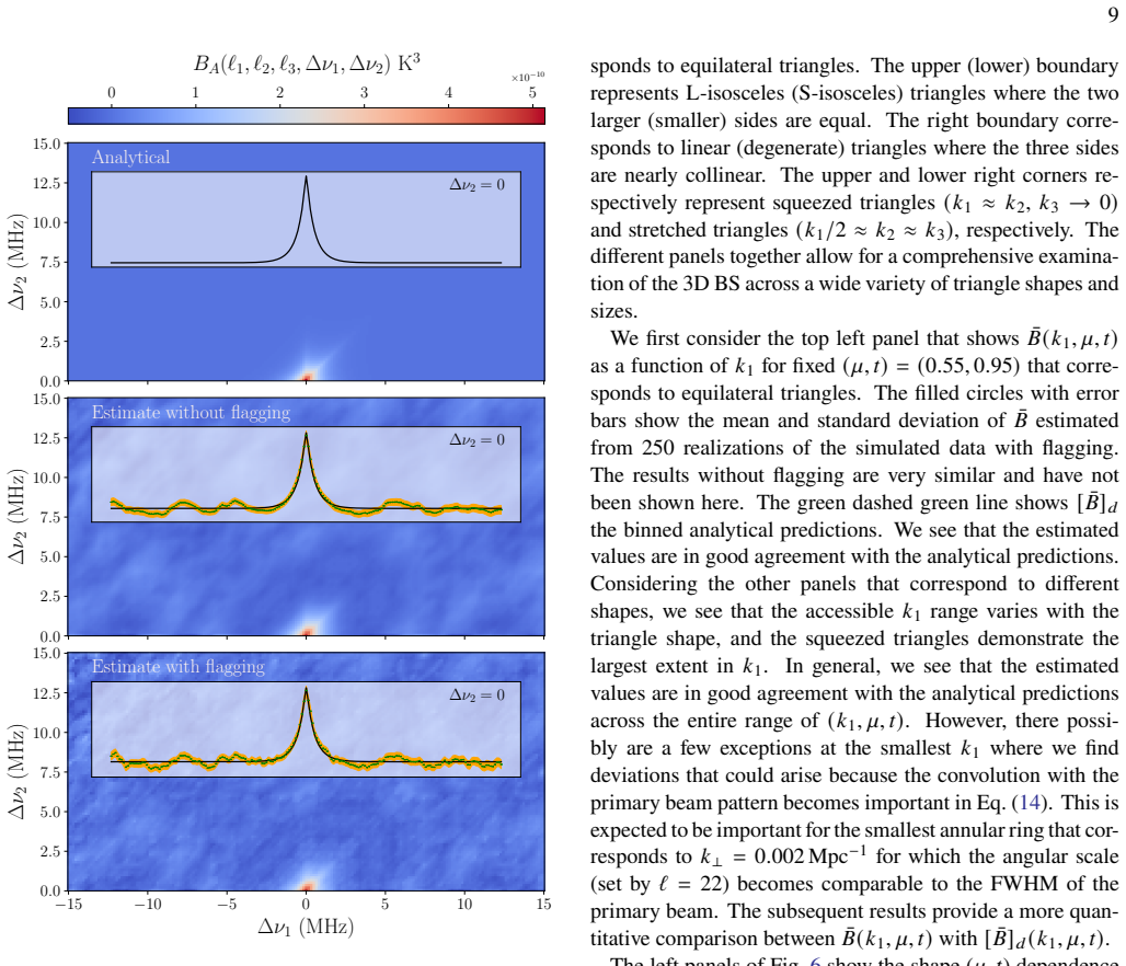
The central object is the binned MABS estimator, Eq. (18): for three annular rings $(a_1,a_2,a_3)$ in three frequency channels, it forms the product $D(\ell_1,\nu_1,\boldsymbol{\theta})D(\ell_2,\nu_2,\boldsymbol{\theta})D(\ell_3,\nu_3,\boldsymbol{\theta})$, where each $D$ is an inverse FFT of the gridded visibilities restricted to one ring, normalizes by the corresponding product of $I$ functions (inverse FFTs of the weighted sampling), and divides by $A=\pi\theta_0^2Q^3/3$. This implements the three-visibility correlation of Eq. (14) that equals the MABS. A 2D DFT over frequency separations, Eq. (19), then maps the MABS to the 3D cylindrical bispectrum $B(k_{1\perp},k_{2\perp},k_{3\perp},k_{1\parallel},k_{2\parallel})$, assuming the signal is ergodic along frequency. The FFT structure reduces the cost from $O(N_c^3 N_t^4)$ to $O(N_c^3 N_t^2 \log N_t^2)$.
What would settle it
Apply the estimator to a simulated 21 cm light cone whose input bispectrum is known to evolve across the band; if the recovered 3D bispectrum deviates from the true band-averaged values by more than the quoted 20 percent, the ergodicity assumption behind the frequency-to-parallel-wavenumber transform is falsified.
Extended reading notes
Core claim
The central claim is that the binned MABS estimator of Eq. (18) — a normalized product of three inverse FFTs of gridded visibilities restricted to annular rings at three frequencies — is an unbiased estimate of the MABS, and that a 2D discrete Fourier transform over frequency separations (Eq. 19) recovers the cylindrical 3D bispectrum under ergodicity along the frequency axis. The validation uses 250 independent realizations of a simulated MWA pointing with a known input bispectrum. The estimated monopole bispectrum agrees with analytical predictions across $0.003\,\mathrm{Mpc}^{-1} \leq k_1 \leq 1.258\,\mathrm{Mpc}^{-1}$ and a wide range of triangle shapes; fractional deviations stay below 20 percent even when the simulated data have exactly the same flagged frequency channels as the actual MWA observations, and most deviations lie within $1\sigma$ to $3\sigma$ of the expected statistical fluctuations.
Load-bearing premise
The method assumes the 21 cm signal is statistically uniform along the frequency axis, so that the 3D bispectrum can be obtained by a 2D Fourier transform over frequency separations; if the signal evolves appreciably across the 30.72 MHz band, that transform introduces a bias.
Editorial extensions
If this is right
- Provides, for the first time, a visibility-based estimator for the binned MABS and the 3D 21 cm bispectrum that covers all triangle configurations, not just equilateral and isosceles shapes.
- Brings the computational cost down to $O(N_c^3 N_t^2 \log N_t^2)$; the full-band MWA simulation analysed here takes about one hour on a 16-core CPU.
- Recovers the bispectrum monopole over $k_1 \in [0.003, 1.258]\,\mathrm{Mpc}^{-1}$ for a wide range of triangle shapes, with fractional deviations below 20 percent even under the periodic flagging pattern of actual MWA data.
- Provides the practical route to measuring the non-Gaussian 21 cm signal from the epoch of reionization with interferometers such as MWA, complementing power-spectrum measurements.
Reading between the lines
- Because the validation box is periodic and statistically homogeneous along frequency, the published claims do not yet cover light-cone evolution; applying the estimator to wide-band real data will likely require splitting the band into redshift windows in which ergodicity approximately holds.
- Foregrounds are absent from this validation. In real data, spectrally smooth foregrounds concentrated in the wedge could still contribute to the FFT products, so foreground avoidance or subtraction will likely be needed before the estimated bispectrum can be interpreted cosmologically.
- Combining this bispectrum estimator with a power-spectrum estimate from the same gridded visibilities could break degeneracies among reionization parameters (for example bubble size versus ionizing efficiency) that the power spectrum alone cannot separate.
- The formalism already yields all non-zero multipole moments of the bispectrum; measuring them on real data would directly probe redshift-space distortions and line-of-sight anisotropy, a step the paper leaves for future work.
Editorial analysis
A structured set of objections, weighed in public.
Referee Report
Summary. The paper extends the single-frequency angular-bispectrum estimator of Paper I to multifrequency observations. It defines a binned estimator for the multi-frequency angular bispectrum (MABS) from gridded visibilities using annular rings and FFTs, and then obtains the 3D 21-cm bispectrum by a 2D DFT over frequency separations under the assumption of frequency ergodicity. The estimator is validated with 250 realizations of a non-Gaussian field with a known analytic bispectrum, using an MWA drift-scan baseline distribution, both with and without the observed flagging pattern. The paper reports agreement with analytic predictions at the ≲20% level over k1 in [0.003, 1.258] Mpc^{-1} and concludes that the deviations are mostly consistent with statistical fluctuations.
Significance. The estimator is a useful step toward measuring 21-cm non-Gaussianity: it is presented as the first visibility-based MABS estimator and it covers all triangle shapes in a binned sense. The validation strategy is honest in an important respect: no free parameters are fitted to the target bispectrum, and the analytical predictions are binned over the same discrete k modes as the estimates. The flagging-robustness test is also valuable. However, two issues currently limit the strength of the central claims: as written, the implemented estimator in Eq. (18) omits the non-closure exponential factor that appears in the defining relation Eq. (14), and the 3D-bispectrum part is validated only under a frequency-stationarity assumption that real light-cone data will violate. Both issues are fixable, but they are load-bearing for the unbiasedness and generalizability claims.
major comments (3)
- [Section 3.2, Eqs. (14) and (18)] Eq. (14) contains the non-closure correction factor exp(π^2 θ0^2 ΔU^2/3), but the implemented binned estimator in Eq. (18) contains only the prefactor 1/A and does not apply this exponential. Section 4 explicitly states that the factor is 0.89 for a typical value of (ΔU)^2 = (ΔU_g)^2/2. If the exponential is not applied, the estimator is biased low by roughly 5–11%, depending on the typical ΔU distribution. This is not negligible relative to the claimed 20% accuracy, and it is a natural explanation for the 4–5σ deviations reported at high k1 in the no-flagging case (Section 5, Figs. 7–8). The authors should include the correction, e.g., as a bin-dependent weight, or quantify its residual effect and show that it is below the statistical error bars.
- [Section 2.2, Eq. (10); Section 4] The 3D BS estimator is built on the assumption that the signal is ergodic along frequency, so that the MABS depends only on (Δν1, Δν2) and Eq. (10) is an exact 2D Fourier relation. The validation in Section 4 uses a periodic 2048^3 box with a statistically homogeneous line of sight, so this assumption is exact by construction and is never stressed. For the real MWA band (ν_c = 154.25 MHz, B_bw = 30.72 MHz, z ≈ 7.4–9.2) the 21 cm signal evolves substantially across the band; under light-cone evolution the MABS depends on absolute frequencies and the recovered k∥ modes become a weighted mix of true modes. Since the headline claim concerns the 3D BS for the EoR, the authors should either add a light-cone simulation test that quantifies the bias, or explicitly restrict the 3D BS claim to a regime where frequency ergodicity holds and discuss the expected bias on the full band.
- [Section 5, Figs. 7 and 8] The text states that for the largest k1 bins (0.413–1.258 Mpc^{-1}) and linear triangles, most no-flagging estimates have 4 < Δσ ≤ 5, while the flagged case shows smaller Δσ. With 250 independent realizations, many 4–5σ deviations in a single configuration are not plausibly statistical, and the decrease of Δσ when flagging is added suggests a fixed systematic offset rather than a purely statistical effect. The conclusion that the deviations are 'mostly consistent with the expected statistical fluctuations' needs quantitative support: the authors should report the full Δσ distribution, test whether the analytic binning uses the same effective weights as the estimator (especially near degenerate/linear triangles where B̄ varies rapidly within a bin), and either correct or explicitly exclude the discrepant bins.
minor comments (6)
- [Section 4] The cosmological parameters used to evaluate r and r' are not stated, although all k⊥ and k∥ values quoted in Section 5 depend on them.
- [Section 5, Fig. 5 caption] Calling (μ, t) = (0.55, 0.95) 'equilateral' is imprecise; the exact equilateral configuration is (μ, t) = (0.5, 1). Please refer to this bin as the one nearest to equilateral.
- [Section 4] The statement that U = 250 corresponds to an angular scale of 0.115° appears to be off by a factor of two; for a baseline U, the angular scale is approximately 1/U in radians, i.e., about 0.23° for U = 250.
- [Section 3.2 and Section 6] The claimed computational complexity O(N_c^3 N_t^2 log N_t^2) omits the number of radial rings N_r; the triple-ring combinations in Eq. (18) contribute an additional factor N_r^3, which should be stated.
- [Section 4] The description of the flagging after collapsing four frequency channels is ambiguous when a collapsed block is only partially flagged; please specify how such blocks are treated.
- [Figs. 7 and 8 captions] The definition of Δσ in the captions is written as '|B̄ − [B̄]_d/σ', with the absolute value left open; it should read '|B̄ − [B̄]_d|/σ'.
Circularity Check
No significant circularity: the estimator is validated against a known input model with no fitted constants, and the analytic predictions are the input bispectrum rather than products of the estimator.
full rationale
The paper's derivation chain is self-contained as an estimator test. Section 3 defines the binned MABS estimator (Eq. 18) as a normalized triple product of FFTs of gridded visibilities; no parameter is fitted to the simulated data. The analytic reference in Section 4 is computed directly from the input model: the non-Gaussian field is generated by Eq. (20) with P(k)=k^{-2}, and Eq. (21) gives the corresponding input bispectrum to first order in f_NG. The 'analytical predictions' are therefore the known ground truth of the simulation, not a quantity derived from the estimator. The MABS analytic prediction is obtained by inverting Eq. (10), which is the same Fourier relation used to form the 3D BS; this is a consistency check of the transform pair, not a reduction of the estimator to its input. The validation uses a periodic, statistically homogeneous line of sight, so the frequency-ergodicity assumption underlying Eq. (10) is satisfied by construction; the paper explicitly notes that the MABS itself does not require ergodicity (Sections 1 and 2.2). The light-cone evolution of a real 30.72 MHz band is not tested, and the paper lists foregrounds, noise, and systematics as omissions (Section 6); these are limitations for future work, not circular steps. Self-citations to Paper I (Gill et al. 2025) for the single-frequency visibility estimator are normal and are supported by the current end-to-end simulation validation.
Assumptions & free parameters
free parameters (2)
- f_NG =
1
- annular ring binning scheme =
22 rings with widths increasing from 4 (U=1 to 5) to two rings (U=200 to 250)
assumptions (6)
- domain assumption Statistical homogeneity and isotropy of the brightness temperature field in the plane of the sky.
- domain assumption Ergodicity of the signal along the frequency (line-of-sight) direction.
- domain assumption Flat-sky approximation with a Gaussian primary beam and fixed Q and theta_0 across the band.
- domain assumption The analytic bispectrum is valid to first order in f_NG and requires f_NG sigma_T << 1.
- standard math Discrete Fourier transforms on the gridded visibilities faithfully represent the required continuous Fourier integrals.
- domain assumption The validation can ignore system noise, astrophysical foregrounds, and instrumental systematics.
Cite this review
Pith. "Pith review of A Visibility-based 21 cm Bispectrum Estimator for Radio-interferometric Data." pith.science (2026). https://pith.science/paper/YR5KDN2A
@misc{pith2026250610526,
  author       = {Pith},
  title        = {Pith review of: A Visibility-based 21 cm Bispectrum Estimator for Radio-interferometric Data},
  year         = {2026},
  howpublished = {\url{https://pith.science/paper/YR5KDN2A}},
  note         = {Machine review of arXiv:2506.10526}
}
abstract
We present a fast and scalable estimator for the binned multi-frequency angular bispectrum (MABS) and the 3D bispectrum (BS) of the redshifted 21 cm signal from radio interferometric observations. The estimator operates on gridded visibilities and leverages the FFT-based acceleration to efficiently compute the MABS and the 3D BS covering all possible triangle configurations. We present the formalism and validate the estimator using simulated visibility data for a known input model BS, considering the Murchison Widefield Array (MWA) observations with a bandwidth of $30.72$ MHz centered at $154.25$ MHz. We consider two cases, namely, without flagging, and with flagging, which has exactly the same frequency channels flagged as the actual data. We obtain estimates of the BS for a wide range of triangle shapes covering the scales $0.003 ~\mathrm{Mpc}^{-1}\leq k_1 \leq 1.258 ~\mathrm{Mpc}^{-1}$. The estimated BS shows excellent agreement with analytical predictions based on the input model BS. We find that the deviations, which are below 20\% even in the presence of flagging, are mostly consistent with the expected statistical fluctuations. This work paves the way for reliable observational estimates of the 21 cm BS for the epoch of reionization, where the signal is predicted to be highly non-Gaussian.
Figures


Figures from the paper (5 more)


Reference graph
Works this paper leans on
-
[1]
, " * write output.state after.block = add.period write newline
ENTRY address archivePrefix author booktitle chapter doi edition editor eprint howpublished institution journal key month number organization pages publisher school series title misctitle type volume year version url label extra.label sort.label short.list INTEGERS output.state before.all mid.sentence after.sentence after.block FUNCTION init.state.consts ...
-
[2]
write newline
" write newline "" before.all 'output.state := FUNCTION format.url url empty "" new.block "" url * "" * if FUNCTION format.eprint eprint empty "" archivePrefix empty "" archivePrefix "arXiv" = new.block " " eprint * " " * new.block " " eprint * " " * if if if FUNCTION format.doi doi empty "" " " doi * " " * if FUNCTION format.pid doi empty eprint empty ur...
-
[3]
Ք[J.XC72qM싕-b̪q) , d,q] fY`I WH R0 [6Yp 6`H
thebibliography [1] 20pt to REFERENCES 6pt =0pt -12pt 10pt plus 3pt =0pt =0pt =1pt plus 1pt =0pt =0pt -12pt =13pt plus 1pt =20pt =13pt plus 1pt \@M =10000 =-1.0em =0pt =0pt 0pt =0pt =1.0em @enumiv\@empty 10000 10000 `\.\@m \@noitemerr \@latex@warning Empty `thebibliography' environment \@ifnextchar \@reference \@latexerr Missing key on reference command E...
-
[4]
S., Bharadwaj , S., & Chengalur , J
Ali , S. S., Bharadwaj , S., & Chengalur , J. N. 2008, , 385, 2166, 10.1111/j.1365-2966.2008.12984.x
arXiv 2008
-
[6]
2019, , 485, 2235, 10.1093/mnras/stz532
Bag , S., Mondal , R., Sarkar , P., et al. 2019, , 485, 2235, 10.1093/mnras/stz532
-
[7]
2018, , 477, 1984, 10.1093/mnras/sty714
Bag , S., Mondal , R., Sarkar , P., Bharadwaj , S., & Sahni , V. 2018, , 477, 1984, 10.1093/mnras/sty714
-
[9]
Bharadwaj , S., & Ali , S. S. 2005, , 356, 1519, 10.1111/j.1365-2966.2004.08604.x
arXiv 2005
-
[10]
2020, , 493, 594, 10.1093/mnras/staa279
Bharadwaj , S., Mazumdar , A., & Sarkar , D. 2020, , 493, 594, 10.1093/mnras/staa279
Show all 61 references
-
[11]
2019, , 483, 5694, 10.1093/mnras/sty3501
Bharadwaj , S., Pal , S., Choudhuri , S., & Dutta , P. 2019, , 483, 5694, 10.1093/mnras/sty3501
2019 doi
-
[12]
Bharadwaj , S., & Pandey , S. K. 2005, , 358, 968, 10.1111/j.1365-2966.2005.08836.x
2005
-
[13]
Bharadwaj , S., & Sethi , S. K. 2001, Journal of Astrophysics and Astronomy, 22, 293, 10.1007/BF02702273
2001 doi
-
[14]
Chatterjee , S., Bharadwaj , S., Choudhuri , S., Sethi , S., & Patwa , A. K. 2023, , 519, 2410, 10.1093/mnras/stac3576
2023 doi
-
[15]
Chatterjee , S., Elahi , K. M. A., Bharadwaj , S., et al. 2024, , 41, e077, 10.1017/pasa.2024.45
2024 doi
-
[16]
2022, , 261, 29, 10.3847/1538-4365/ac6fd9
CHIME Collaboration , Amiri , M., Bandura , K., et al. 2022, , 261, 29, 10.3847/1538-4365/ac6fd9
2022 doi
-
[17]
Choudhuri , S., Bharadwaj , S., Ghosh , A., & Ali , S. S. 2014, , 445, 4351, 10.1093/mnras/stu2027
2014 doi
-
[18]
2008, , 77, 103506, 10.1103/PhysRevD.77.103506
Cooray , A., Li , C., & Melchiorri , A. 2008, , 77, 103506, 10.1103/PhysRevD.77.103506
2008 doi
-
[19]
2021, arXiv e-prints, arXiv:2102.11153
Cunnington , S., Watkinson , C., & Pourtsidou , A. 2021, arXiv e-prints, arXiv:2102.11153. 2102.11153
2021 arXiv
-
[20]
2023, , 523, 2453, 10.1093/mnras/stad1567
Cunnington , S., Wolz , L., Bull , P., et al. 2023, , 523, 2453, 10.1093/mnras/stad1567
2023 doi
-
[21]
D., & Carilli , C
Datta , A., Bowman , J. D., & Carilli , C. L. 2010, , 724, 526, 10.1088/0004-637X/724/1/526
2010 doi
-
[22]
K., Choudhury , T
Datta , K. K., Choudhury , T. R., & Bharadwaj , S. 2007, , 378, 119, 10.1111/j.1365-2966.2007.11747.x
2007
-
[23]
R., Parsons , A
DeBoer , D. R., Parsons , A. R., Aguirre , J. E., et al. 2017, , 129, 045001, 10.1088/1538-3873/129/974/045001
2017 doi
-
[24]
2020, JCAP, 12, 003, 10.1088/1475-7516/2020/12/003
Durrer, R., Jalilvand, M., Kothari, R., Maartens, R., & Montanari, F. 2020, JCAP, 12, 003, 10.1088/1475-7516/2020/12/003
2020 doi
- [25]
-
[26]
Elahi , K. M. A., Bharadwaj , S., Pal , S., et al. 2023, , 525, 3439, 10.1093/mnras/stad2495
2023 doi
-
[27]
2024 b , , 529, 3372, 10.1093/mnras/stae740
---. 2024 b , , 529, 3372, 10.1093/mnras/stae740
2024 doi
-
[28]
S., & Chengalur, J
Ghosh, A., Bharadwaj, S., Ali, S. S., & Chengalur, J. N. 2011, Monthly Notices of the Royal Astronomical Society, 411, 2426, 10.1111/j.1365-2966.2010.17853.x
2011
- [29]
-
[30]
S., Bharadwaj, S., Ali, S
Gill, S. S., Bharadwaj, S., Ali, S. S., & Elahi, K. M. A. 2025, Astrophys. J., 979, 25, 10.3847/1538-4357/ad9b20
2025 doi
-
[31]
S., Pramanick , S., Bharadwaj , S., Shaw , A
Gill , S. S., Pramanick , S., Bharadwaj , S., Shaw , A. K., & Majumdar , S. 2024, , 527, 1135, 10.1093/mnras/stad3273
2024 doi
-
[32]
S., et al
Gupta , Y., Ajithkumar , B., Kale , H. S., et al. 2017, Current Science, 113, 707
2017
-
[33]
Hamilton , A. J. S. 1998, in Astrophysics and Space Science Library, Vol. 231, The Evolving Universe, ed. D. Hamilton , 185, 10.1007/978-94-011-4960-0_17
1998 doi
-
[34]
A., Seiler, J., et al
Hutter, A., Watkinson, C. A., Seiler, J., et al. 2020, Mon. Not. Roy. Astron. Soc., 492, 653, 10.1093/mnras/stz3139
2020 doi
-
[35]
2010, PhD thesis, Cosmology with high (z > 1) redshift galaxy surveys, Univ
Jeong, D. 2010, PhD thesis, Cosmology with high (z > 1) redshift galaxy surveys, Univ. Texas at Austin
2010
-
[36]
2021, , 502, 3800, 10.1093/mnras/stab216
Kamran , M., Ghara , R., Majumdar , S., et al. 2021, , 502, 3800, 10.1093/mnras/stab216
2021 doi
-
[37]
Karagiannis , D., Maartens , R., & Randrianjanahary , L. F. 2022, , 2022, 003, 10.1088/1475-7516/2022/11/003
2022 doi
-
[38]
Line , J. L. B., McKinley , B., Rasti , J., et al. 2018, , 35, e045, 10.1017/pasa.2018.30
2018 doi
-
[39]
R., et al
Majumdar, S., Kamran, M., Pritchard, J. R., et al. 2020, Mon. Not. Roy. Astron. Soc., 499, 5090, 10.1093/mnras/staa3168
2020 doi
-
[40]
R., Mondal, R., et al
Majumdar, S., Pritchard, J. R., Mondal, R., et al. 2018, Mon. Not. Roy. Astron. Soc., 476, 4007, 10.1093/mnras/sty535
2018 doi
-
[41]
2020, , 498, 3975, 10.1093/mnras/staa2548
Mazumdar , A., Bharadwaj , S., & Sarkar , D. 2020, , 498, 3975, 10.1093/mnras/staa2548
2020 doi
-
[42]
F., Hazelton , B., Sullivan , I., & Beardsley , A
Morales , M. F., Hazelton , B., Sullivan , I., & Beardsley , A. 2012, , 752, 137, 10.1088/0004-637X/752/2/137
2012 doi
-
[43]
2020, Monthly Notices of the Royal Astronomical Society, 10.1093/mnras/staa3831
Pal, S., Bharadwaj, S., Ghosh, A., & Choudhuri, S. 2020, Monthly Notices of the Royal Astronomical Society, 10.1093/mnras/staa3831
2020 doi
-
[44]
R., Pober, J
Parsons, A. R., Pober, J. C., Aguirre, J. E., et al. 2012, The Astrophysical Journal, 756, 165, 10.1088/0004-637x/756/2/165
2012 doi
-
[45]
K., Sethi , S., & Dwarakanath , K
Patwa , A. K., Sethi , S., & Dwarakanath , K. S. 2021, , 504, 2062, 10.1093/mnras/stab989
2021 doi
- [46]
-
[47]
2007, , 662, 1, 10.1086/517963
Pillepich , A., Porciani , C., & Matarrese , S. 2007, , 662, 1, 10.1086/517963
2007 doi
-
[48]
F., Karagiannis , D., & Maartens , R
Randrianjanahary , L. F., Karagiannis , D., & Maartens , R. 2024, Physics of the Dark Universe, 45, 101530, 10.1016/j.dark.2024.101530
2024
-
[49]
A., Keating , L
Raste , J., Kulkarni , G., Watkinson , C. A., Keating , L. C., & Haehnelt , M. G. 2024, , 529, 129, 10.1093/mnras/stae492
2024 doi
-
[50]
2019, Mon
Sarkar, D., Majumdar, S., & Bharadwaj, S. 2019, Mon. Not. Roy. Astron. Soc., 490, 2880, 10.1093/mnras/stz2799
2019 doi
-
[51]
2020, Mon
Saxena, A., Majumdar, S., Kamran, M., & Viel, M. 2020, Mon. Not. Roy. Astron. Soc., 497, 2941, 10.1093/mnras/staa1768
2020 doi
-
[52]
2015, , 92, 083532, 10.1103/PhysRevD.92.083532
Scoccimarro , R. 2015, , 92, 083532, 10.1103/PhysRevD.92.083532
2015 doi
-
[53]
Scoccimarro , R., Couchman , H. M. P., & Frieman , J. A. 1999, , 517, 531, 10.1086/307220
1999 doi
-
[54]
2005, PhD thesis, Probing fundamental physics with large-scale structure: From galaxy formation to inflation, Polytechnic University, United States
Sefusatti , E. 2005, PhD thesis, Probing fundamental physics with large-scale structure: From galaxy formation to inflation, Polytechnic University, United States
2005
-
[55]
2006, , 74, 023522, 10.1103/PhysRevD.74.023522
Sefusatti , E., Crocce , M., Pueblas , S., & Scoccimarro , R. 2006, , 74, 023522, 10.1103/PhysRevD.74.023522
2006 doi
-
[56]
K., Bharadwaj , S., Sarkar , D., et al
Shaw , A. K., Bharadwaj , S., Sarkar , D., et al. 2021, arXiv e-prints, arXiv:2107.14564. 2107.14564
2021 arXiv
-
[57]
2017, Mon
Shimabukuro, H., Yoshiura, S., Takahashi, K., Yokoyama, S., & Ichiki, K. 2017, Mon. Not. Roy. Astron. Soc., 468, 1542, 10.1093/mnras/stx530
2017 doi
-
[58]
J., Goeke , R., Bowman , J
Tingay , S. J., Goeke , R., Bowman , J. D., et al. 2013, , 30, e007, 10.1017/pasa.2012.007
2013 doi
-
[59]
M., et al
Trott, C. M., et al. 2019, Publ. Astron. Soc. Austral., 36, e023, 10.1017/pasa.2019.15
2019 doi
-
[60]
van Haarlem, M. P. , Wise, M. W. , Gunst, A. W. , et al. 2013, A&A, 556, A2, 10.1051/0004-6361/201220873
2013 doi
-
[61]
A., Giri, S
Watkinson, C. A., Giri, S. K., Ross, H. E., et al. 2019, Mon. Not. Roy. Astron. Soc., 482, 2653, 10.1093/mnras/sty2740
2019 doi
-
[62]
A., Greig , B., & Mesinger , A
Watkinson , C. A., Greig , B., & Mesinger , A. 2022, , 510, 3838, 10.1093/mnras/stab3706
2022 doi
-
[63]
A Simplified, Lossless Reanalysis of PAPER-64
Koopmans L., et al., 2015, aska.conf, 1, aska.conf @ARTICLE Kolopanis19, author = Kolopanis , Matthew and Jacobs , Daniel C. and Cheng , Carina and Parsons , Aaron R. and Kohn , Saul A. and Pober , Jonathan C. and Aguirre , James E. and Ali , Zaki S. and Bernardi , Gianni and ...
2015 arXiv
Reviewed August 7, 2026 · model on record in the stance chip above.
Discussion (0). Continue with ORCID to comment.