Spatial and Temporal fluctuation of an ABP in an optical trap

Chong Shen; H.Daneil Ou-Yang; Lanfang Li; Zhiyu Jiang

REVIEW 3 major objections 5 minor 37 references

Spatial and Temporal fluctuation of an ABP in an optical trap

T0 review · 3 major / 5 minor · reviewed 2026-08-14 · deepseek-v4-flash

Challenge this review Re-run · record.json Download PDF Read on arXiv ↗ Review JSON

Pith's one-line read The power spectrum of a trapped active particle is a Brownian spectrum plus a Lorentzian bump whose height encodes swim speed and rotational diffusion.

desk verdict A well-constructed experimental ABP-in-trap study with a correct HPP convolution analysis, but Eq 10's factor-2π corner error invalidates the paper's central quantitative PSD claim. read the letter →

arxiv 1908.08157 v2 pith:YSDW5P4S submitted 2019-08-22 cond-mat.soft physics.optics

Chong Shen , Lanfang Li , Zhiyu Jiang , H.Daneil Ou-Yang This is my paper · ORCID

classification cond-mat.softphysics.optics

keywords activeBrownianparticleopticaltrappowerspectraldensitypositionhistograminduced-chargeelectrophoresisJanuseffectivetemperaturerotationaldiffusion

verification ladder T0 review T1 audit T2 compute T3 formal

The pith

A machine-rendered reading of the paper's core claim, the machinery that carries it, and where it could break.

The reading

Using a single metallic Janus particle driven by induced-charge electrophoresis and held in an optical trap, the paper claims that a trapped active Brownian particle's fluctuations factor into a thermal part and an active part, in both space and time. Spatially, the position histogram is the convolution of a Gaussian thermal distribution with an active-only distribution, which is why the histogram splits from one peak to two as the swim speed grows. Temporally, the power spectral density is the Brownian trap spectrum times a one-plus-Lorentzian ratio whose plateau height is set by $v_0^2\tau_r/(2D_t)$ and whose corner frequency is set by the rotational diffusion rate. If the claim is right, a single trapped-particle measurement can yield the swim speed and rotational relaxation directly, and the integrated-spectrum effective temperature should not be treated as a universal measure of dissipation because it depends on trap stiffness.

What carries the argument

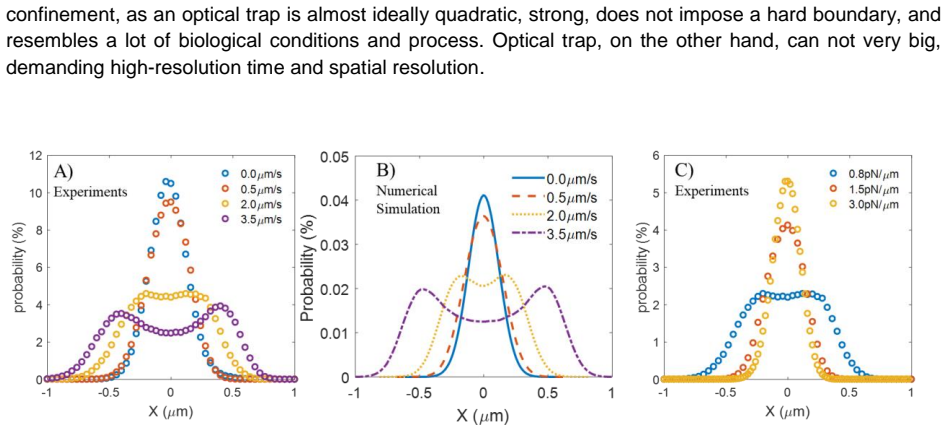
The load-bearing object is the normalized power-spectral-density ratio of Eq. 10, a one-plus-Lorentzian form that attaches the active swim speed to the low-frequency plateau and the rotational diffusion coefficient to the corner frequency. Around it, the paper builds a three-length-scale criterion: the force-balance length $l_1 = v_0\eta/k_{\mathrm{OT}}$, the thermal width $l_2 = \sqrt{k_BT/k_{\mathrm{OT}}}$, and the persistence length $l_3 = v_0/D_r$; their ratios decide whether the position histogram stays Gaussian, flattens, or becomes bimodal. The convolution identity $P(r) = P_A * P_T(r)$ is what lets the paper decouple active and thermal contributions in space, while the PSD ratio decouples them in time.

What would settle it

Perform the same PSD measurement at zero applied voltage while imposing a slow stage drift; if the low-frequency plateau rises above the Brownian baseline without any active swim speed, then drift alone can mimic the Eq. 10 signature. A cleaner quantitative test is to compare the swim speed fitted from the plateau height with the independently measured free-space MSD swim speed: systematic disagreement at low voltage would show the plateau is contaminated.

Watch

Extended reading notes

Core claim

The paper's central result is that the steady-state fluctuations of an active Brownian particle in a quadratic trap separate into a passive part and an active part. In the frequency domain, the normalized power spectrum is $$\frac{S_{\mathrm{active}}(\omega)}{S_{\mathrm{Brownian}}(\omega)} = 1 + \frac{$v_0^{2}$\tau_r/(2D_t)}{(\omega/\omega_r)^2 + 1}, \qquad \omega_r = 2\pi D_r,$$ so the active contribution is a Lorentzian added to the Brownian baseline, with the low-frequency plateau height controlled by the free-space swim speed $v_0$ and rotational relaxation time $\tau_r = 1/D_r$. In real space, the full position distribution is the convolution of the thermal Gaussian and the distribution of a purely active particle in the same trap; the crossover from a single peak to a bimodal distribution is governed by three length scales ($v_0\eta/k_{\mathrm{OT}}$, $\sqrt{k_BT/k_{\mathrm{OT}}}$, $v_0/D_r$) and a critical swim speed. The paper also argues that the integrated PSD and the integrated histogram give the same mean potential energy, but that this integrated quantity is trap-stiffness dependent and therefore should not be interpreted as a universal dissipation or effective temperature.

Load-bearing premise

The claim rests on the low-frequency plateau being real active-particle signal; if slow instrumental drift seeps into that plateau, the fitted swim speed and the effective-temperature comparison lose quantitative support.

Editorial extensions

If this is right

The low-frequency plateau of the PSD ratio directly measures $v_0^2\tau_r/(2D_t)$, so the swim speed can be read from the spectrum without tracking the particle's free-space trajectory.
Because the Brownian baseline is identical at high frequency, the active contribution can be isolated by subtracting the passive spectrum from the active spectrum at each frequency.
The shape of the position histogram is governed by the two ratios $l_1/l_2$ and $l_1/l_3$, so increasing trap stiffness at fixed swim speed pushes a bimodal histogram back toward Gaussian.
The integrated PSD and the integrated histogram yield the same mean potential energy, giving a common measure that links spatial and temporal fluctuation data.
The trap-stiffness dependence of the integrated PSD means it cannot be used as a universal dissipation or effective temperature for active matter without specifying the confinement.

Reading between the lines

Editorial extensions of the paper, not claims the author makes directly.

If Eq. 10 survives drift-control checks, the same trapped-particle setup could serve as a self-calibrating probe: two PSD ratio values at known frequencies would determine both $v_0$ and $D_r$ in a single run.
The one-plus-Lorentzian structure may persist for weakly anharmonic traps, with the effective trap curvature sampled by the particle replacing $k_{\mathrm{OT}}$; checking this would separate geometry effects from genuine active dynamics.
The convolution decomposition suggests a practical assay for weak activity in biological samples: calibrate the passive trap response, then infer the active-only distribution from the difference between measured and convolved histograms.

Share X Bluesky LinkedIn Reddit HN

Signed reviews

No signed human review yet.

Editorial analysis

A structured set of objections, weighed in public.

Desk editor's note, referee report, and a circularity audit.

Desk Editor's Note

read the letter

Colleague,

The paper is worth a look for the experiment, but the central quantitative PSD claim is wrong. The ICEP Janus particle in a quadratic optical trap is a genuinely nice system: large dynamic range, clean optical forces, and a parameter-free Langevin simulation that reproduces the bimodal histograms. The convolution decomposition in Eqs 5–7 is exact for the linear overdamped equation, and the demonstration that the full HPP is the convolution of thermal and active contributions is a solid, well-illustrated point. I give them full credit for that portion.

The problem is Eq 10. From their own Eq 2, the active orientational noise has autocorrelation ~ e^{-D_r t}, so in angular frequency the active contribution to the PSD ratio is Lorentzian with corner at ω = D_r, not at 2πD_r. The paper's ω_r = 2πD_r places the corner a factor 2π too high. This is not a convention issue: Eq 8 uses an angular-frequency Fourier transform, so Eq 10 is internally inconsistent. Even with perfect data and unaffected by drift, the claimed quantitative connection between the PSD corner and the rotational diffusion time would not hold. That is a load-bearing error for the paper's 'two characteristic frequencies' narrative.

Other soft spots are secondary. The low-frequency PSD is drift-prone, as the authors themselves note (with two dangling '[reference needed]' placeholders, which should have been filled before submission). The claim to be the first to see boundary accumulation in an optical trap is overstated, given prior bacterial and acoustic-trap work. The dissipation-fraction interpretation in Fig 6B is muddled. And the figures lack error bars throughout.

What is actually new: the experimental combination of ICEP with simultaneous optical trapping and QPD tracking, and the explicit convolution-based decomposition of the HPP into thermal and active components. That part is publishable. The PSD analysis, as written, is not.

For a peer-review decision: I would send it out despite the flaw, because the system and the HPP convolution are worth refereeing and the PSD error is correctable. But I would tell the authors that Eq 10 must be fixed (ω_r → D_r or an appropriate redefinition and re-fit), the drift issue must be addressed quantitatively, and the novelty claim toned down. If the experiment genuinely shows a corner at the corrected location, the paper becomes a solid contribution. As is, I would not cite the PSD formula, though I might cite the system.

Bring to reading group? Maybe, as a cautionary tale in internal consistency checks.

Best, [Your name]

Referee Report

3 major / 5 minor

Summary. The manuscript reports experiments and numerical simulations of a single induced-charge electrophoretic Janus particle confined in an optical trap, used as a model active Brownian particle. The authors measure position histograms and power spectral densities at controlled active speeds and trap stiffnesses, observing a Gaussian-to-bimodal transition in the histogram and a low-frequency rise in the PSD. They propose a convolution decomposition of thermal and active contributions to the histogram, introduce characteristic length scales and a critical active speed, and claim that the PSD ratio between active and Brownian particles has the Lorentzian form of Eq. (10), with a low-frequency plateau related to the free-space swim speed and a corner frequency set by the rotational diffusion time. They also compare effective temperatures defined from spatial and temporal fluctuations and discuss limitations of classical thermodynamic interpretations in active systems.

Significance. If the claims hold, the paper provides a well-controlled experimental model system with a large dynamic range, and its convolution method for separating thermal and active contributions is a clean consequence of the linearity of the overdamped Langevin equation. The simulations are presented as parameter-free, using independently measured v0, D_t, D_r, and trap stiffness, and the reported Gaussian-to-bimodal HPP transition is consistent with the ABP physics in confinement. The proposed PSD ratio formula, if correctly specified, would be a useful quantitative tool connecting confined temporal fluctuations to the free-space active parameters. These strengths make the core experimental platform valuable. However, the central quantitative PSD claim in Eq. (10) is currently undermined by an internal frequency-convention inconsistency, and the paper itself admits a drift sensitivity that directly affects the low-frequency data used to test that formula.

major comments (3)

[§3.3, Eq. (10)] The corner frequency in Eq. (10) is internally inconsistent with the manuscript's own Langevin model. Equation (8) defines omega as an angular frequency through the exponential e^{i omega (t-t')}. For the overdamped equation Eq. (2), the orientational noise has autocorrelation <cos(theta(t)) cos(theta(0))> = (1/2) e^{-D_r |t|}, whose PSD is proportional to D_r/(D_r^2 + omega^2). Since the same harmonic trap filters both active and passive position signals, the ratio of active to Brownian PSD should be S_ratio(omega) = 1 + [v0^2/(2 D_t)] [D_r^2/(D_r^2 + omega^2)], with the corner at angular frequency omega = D_r. Equation (10) instead places the corner at omega_r = 2 pi D_r, a factor 2 pi higher. If omega in Eq. (10) were intended to be a cyclic frequency, that would contradict the convention used in Eq. (8). Either way, the quantitative statement that the PSD reveals the rotational diffusion time scale through Eq. (10) is not supported as written. This is a load-bearing issue because the 'characteristic frequency' claim and the extraction of tau_r from the PSD depend on this formula.
[§3.3, Fig. 5] The manuscript states in Section 3.3 that 'PSD measurement is highly sensitive to drift noise and at the low frequency (long time scale), the slow drift bias may affect the experimental precision [reference needed].' The low-frequency plateau of the PSD is exactly the region used to test Eq. (10) and to define the zero-frequency effective temperature in Fig. 6. Because drift contamination can raise the low-frequency spectral power, the observed agreement between the experimental PSD ratio and Eq. (10) does not by itself establish the quantitative connection to v0, tau_r, and D_t. The authors need either to demonstrate that drift is negligible in their measured low-frequency data, to correct for drift, or to explicitly restrict the quantitative claim to drift-free simulations.
[§3.3, Eq. (10) and Fig. 5D] Equation (10) is introduced as an ansatz ('We can then write') with no derivation from Eq. (2). The manuscript cites Szamel's work for a similar expression, but that work is for the active component only and does not include the thermal baseline. A direct derivation from the linear Langevin equation is straightforward, as outlined in the first comment, and it yields a different corner frequency. The authors should provide the derivation or at least correct the frequency conventions and verify that the simulation data actually match the corrected Lorentzian form. Without this, the claimed quantitative agreement between Eq. (10) and the simulation data is not credible.

minor comments (5)

[Throughout] There are numerous typographical and grammatical errors that should be fixed: 'Langevine' for Langevin, 'Jans' for Janus, 'serval' for several, 'microecology' likely for micro-rheology, 'the MSD vs time graph appear s', and 'showing in Fig.1 B)' should be 'as shown in Fig. 1B'. These do not affect the science but reduce readability.
[§3.3] Two places in Section 3.3 contain the placeholder '[reference needed]' for statements about drift sensitivity and integration time. These should be supplied or the statements should be removed.
[§3.3, Eq. (9)] Equation (9) appears to be dimensionally inconsistent for a position PSD. The numerator 12 pi eta R k_B times T and the denominator ((k_OT/R)^2 + (eta omega)^2) do not yield units of position power spectral density (m^2 s for angular frequency). This may be a typesetting error (perhaps a missing factor or an incorrect grouping), but it should be corrected because Eq. (9) is presented as the theoretical Brownian PSD reference.
[§2.4 and §3.1] Equation (2) contains 'v0 D' in the active term, which is likely a typo for 'v0 theta_hat' or 'F0 theta_hat' given the form of Eq. (1). In addition, the description of the MSD slopes in Section 3.1 is confusing: the text says the short-time slope is 2 while also saying thermal diffusion gives a slope of 1 at very short times. This should be clarified.
[§3.2, Fig. 3] The text references 'Fig 3 C and D' and discusses simulated HPPs, but Fig. 3 appears to contain only panels A and B, and panel C's caption contains a placeholder 'active speed of xxx'. The figure must be completed or the text adjusted accordingly.

Circularity Check

0 steps flagged · score 0.0 of 10

No circularity found: the paper's central predictions use independently measured parameters, a standard Langevin simulation, and exact linearity/Parseval identities.

full rationale

The derivation chain is self-contained rather than circular. Equation 2 is a standard overdamped Langevin equation for an active Brownian particle, and the simulation is run with experimentally measured v0, k_OT, and the drag coefficient, with no fitting to the target PSD or HPP. The HPP convolution in Eq. 7 follows exactly from linearity of Eqs. 5 and 6, since r = r1 + r2, so the histogram of the sum is the convolution of the two independent component histograms; this is a mathematical identity, not a retrofitted explanation. Similarly, Eq. 15 is the Parseval/autocorrelation identity showing that the frequency integral of the PSD equals the mean squared displacement, so the claimed equality between HPP-integral and PSD-integral effective temperatures is exact. Equation 10 uses v0, tau_r, and D_t obtained from free-space MSD measurements; the low-frequency amplitude v0^2 tau_r/(2D_t) is the independently measured long-time diffusivity enhancement, and it is not obtained by fitting the PSD data. The Lorentzian form is an ansatz motivated by Szamel's result, but because its parameters are not extracted from the target quantity, this is a modeling choice, not a fitted-input-called-prediction. The paper does cite the authors' own prior work [19] for Eq. 2, but the equation is standard and is also supported by [28], so the self-citation is not load-bearing. The manuscript itself flags a genuine experimental limitation: 'PSD measurement is highly sensitive to drift noise and at the low frequency ... the slow drift bias may affect the experimental precision [reference needed]' (Section 3.3). That is a data-quality caveat, not circularity. The skeptic's concern that Eq. 10 places the corner at omega_r = 2πD_r rather than D_r is an internal consistency/derivation issue that affects the quantitative claim, but it does not make the argument circular, because the formula is not equivalent to its inputs by construction. Overall, no circular step reduces a claimed prediction to its own input.

Assumptions & free parameters 3 free parameters · 6 assumptions · 0 invented entities

The central claims depend on measured swim parameters (v0, Dr, Dt) and the overdamped Langevin model. No new physical entities are introduced. The main modeling assumption is the ad hoc Lorentzian form of Eq 10, which is not derived and only qualitatively matches the low-frequency data.

free parameters (3)

rotational relaxation time tau_r = 17.8 ± 1.4 s
Fitted from free-space MSD (Eq 4) using data from the same Janus particles; used as input to simulations and in Eq 10 for the PSD ratio.
translational diffusivity D_t = 0.053 ± 0.008 um^2/s
Measured from zero-voltage MSD; used in Eq 10 and in Stokes-Einstein comparisons.
active swim speed v0 = 0 to about 3.5 um/s depending on applied voltage
Obtained from free-space MSD fits (Eq 4) at each applied voltage; used to parameterize simulations and Eq 10.

assumptions (6)

domain assumption The overdamped Langevin equation (Eq 2) with additive white translational noise and independent orientational diffusion describes the Janus particle.
Invoked in Section 2.4 and used for all simulations and analytical expressions.
standard math Active and thermal noises are independent, so the position distribution is the convolution of the two contributions (Eq 7).
The linearity of the Langevin equation implies r = r1 + r2, and independence of the noises gives P = P_A * P_P.
ad hoc to paper The PSD ratio has the Lorentzian form of Eq 10 with parameters from free-space measurements.
Eq 10 is stated without derivation as 'We can then write' after inspecting the data; it is not derived from the Langevin equation.
domain assumption The optical trap is a quadratic potential with stiffness k_OT measured independently.
Used throughout Section 3.2 and 3.3; measured by passive/active microrheology (refs 24,25).
domain assumption The ICEP velocity is proportional to E^2 and constant in time.
Based on theory (ref 29) and verified by the linear v0 vs V^2 relation in Fig 2B.
standard math Parseval's theorem equates the integral of the PSD to the mean-square displacement (Eq 15).
Used in Section 3.4 to connect spatial and temporal effective temperatures.

how reviews work

0 comments

Cite this review

Pith. "Pith review of Spatial and Temporal fluctuation of an ABP in an optical trap." pith.science (2026). https://pith.science/paper/YSDW5P4S

@misc{pith2026190808157,
  author       = {Pith},
  title        = {Pith review of: Spatial and Temporal fluctuation of an ABP in an optical trap},
  year         = {2026},
  howpublished = {\url{https://pith.science/paper/YSDW5P4S}},
  note         = {Machine review of arXiv:1908.08157}
}

read the original abstract

A colloidal suspension of active Brownian particles (ABPs) driven by controllable forces into directed or persistent motions can serve as a model for understanding the biological systems. Experiments and numerical simulations are established to investigate the motions of an ABP, a single, induced-charge electrophoretic (ICEP) metallic Janus particle, confined in a quadratic potential well. On the one hand, 1-D position histograms of the trapped active particle, behaving differently from that of a Boltzmann distribution, reveal a splitting from a single peak of the ABP positional distribution to a bimodal distribution. Decoupling the thermal and non-thermal contributions from the overall histogram is non-trivial. However, the two contributions can be examined by convoluting numerically generated thermal and non-thermal contributions into a full histogram. On the other hand, temporal fluctuations analyzed by the power spectral density (PSD), reveal two unique frequencies characterizing the stiffness of the trap and the rotational diffusion of the particle, respectively. Connections between the spatial and temporal fluctuations are obtained by the separate analysis of the temporal and spatial fluctuations of an ABP trapped in a quadratic potential well. This study reveals how thermal and nonthermal fluctuations play against each other in a confined environment.

Figures

Figures reproduced from arXiv: 1908.08157 by the authors.

**Figure 4.** Numerically simulated histogram of particle position (HPP). Thermal noise (solid blue line), active noise (orange solid line), active +thermal noise (yellow solid line) and the convolution (purple dash line) between the histogram of thermal noise and histogram of active noise. Different dynamic parameters: active speed v, and rotational diffusion coefficient Dr, are shown. A) v=10um/s Dr=3/s B) v=100um/s Dr=500/s C)… view at source ↗

**Figure 5.** FIG. 5. A) Experimental fluctuation power spectral density (PSD) of 3um Janus particles under 1.5pN/um [PITH_FULL_IMAGE:figures/full_fig_p009_5.png] view at source ↗

Figures from the paper (1 more)

**Figure 6.** Figure 6: A) Effective temperature Teff, normalized with ambient temperature, calculated from simulation data with different definitions: a) Teff calculated from potential energy associated with spatial distribution; b) Teff calculated from diffusion coefficient at long time sca…

Discussion (0). Continue with ORCID to comment.

Reference graph

Works this paper leans on

37 extracted references · 36 canonical work pages

[1]

Ramaswamy, Annu

S. Ramaswamy, Annu. Rev. Condens. Matter Phys. (2010)

work page 2010
[2]

Mizuno, C

D. Mizuno, C. Tardin, C. F. Schmidt, and F. C. MacKintosh, Science (80-. ). 315, 370 (2007)

work page 2007
[3]

Fodor, M. Guo, N. S. Gov, P. Visco, D. A. Weitz, and F. Van Wijland, EPL (2015)

work page 2015
[4]

T. Betz, M. Lenz, J. F. Joanny, and C. Sykes, Proc. Natl. Acad. Sci. U. S. A. 106, 15320 (2009)

work page 2009
[5]

Ben-Isaac, E

E. Ben-Isaac, E. Fodor, P. Visco, F. Van Wijland, and N. S. Gov, Phys. Rev. E - Stat. Nonlinear, Soft Matter Phys. (2015)

work page 2015
[6]

Fodor, W. W. Ahmed, M. Almonacid, M. Bussonnier, N. S. Gov, M. H. Verlhac, T. Betz, P. Vis co, and F. Van Wijland, EPL 116, (2016)

work page 2016
[7]

Seifert and T

U. Seifert and T. Speck, EPL 89, (2010)

work page 2010
[8]

Fodor, C

É. Fodor, C. Nardini, M. E. Cates, J. Tailleur, P. Visco, and F. Van Wijland, Phys. Rev. Lett. (2016)

work page 2016

Show all 37 references

[9]

S. C. Takatori and J. F. Brady, Phys. Rev. E - Stat. Nonlinear, Soft Matter Phys. (2015)

2015
[10]

U. Basu, S. N. Majumdar, A. Rosso, and G. Schehr, Phys. Rev. E (2018)

2018
[11]

D. Loi, S. Mossa, and L. F. Cugliandolo, Phys. Rev. E - Stat. Nonlinear, Soft Matter Phys. (2008)

2008
[12]

Palacci, C

J. Palacci, C. Cottin-Bizonne, C. Ybert, and L. Bocquet, Phys. Rev. Lett. (2010)

2010
[13]

Uspal, M

W. Uspal, M. Popescu, S. Dietrich, M. T.-S. Matter, and undefined 2015, Pubs.Rsc.Org (n.d.)

2015
[14]

Bechinger, R

C. Bechinger, R. Di Leonardo, H. Lö wen, C. Reichhardt, G. Volpe, and G. Volpe, Rev. Mod. Phys. (2016)

2016
[15]

D. Ray, C. Reichhardt, and C. J. O. Reichhardt, Phys. Rev. E - Stat. Nonlinear, Soft Matter Phys. (2014)

2014
[16]

Frydel and R

D. Frydel and R. Podgornik, Phys. Rev. E (2018)

2018
[17]

S. C. Takatori, R. De Dier, J. Vermant, and J. F. Brady, Nat. Commun. (2016)

2016
[18]

Argun, A

A. Argun, A. R. Moradi, E. Pinç e, G. B. Bagci, A. Imparato, and G. Volpe, Phys. Rev. E (2016)

2016
[19]

H. D. Ou-Yang and C. Shen, in (2018)

2018
[20]

Jiang, Q

S. Jiang, Q. Chen, M. Tripathy, E. Luijten, K. S. Schweizer, and S. Granick, Adv. Mater. (2010)

2010
[21]

Muangnapoh, A

T. Muangnapoh, A. L. Weldon, and J. F. Gilchrist, Appl. Phys. Lett. (2013)

2013
[22]

Gangwal, O

S. Gangwal, O. J. Cayre, M. Z. Bazant, and O. D. Velev, Phys. Rev. Lett. (2008)

2008
[23]

I. F. Sbalzarini and P. Koumoutsakos, J. Struct. Biol. (2005)

2005
[24]

M. T. Valentine, L. E. Dewalt, and H. D. Ou-Yang, J. Phys. Condens. Matter (1996)

1996
[25]

M.-T. Wei, A. Zaorski, H. C. Yalcin, J. Wang, M. Hallow, S. N. Ghadiali, A. Chiou, and H. D. Ou - Yang, Opt. Express (2008)

2008
[26]

Y. Zong, J. Liu, R. Liu, H. Guo, M. Yang, Z. Li, and K. Chen, ACS Nano (2015)

2015
[27]

Nedev, S

S. Nedev, S. Carretero-Palacios, P. Kü hler, T. Lohmü ller, A. S. Urban, L. J. E. Anderson, and J. Feldmann, ACS Photonics (2015)

2015
[28]

Volpe, S

G. Volpe, S. Gigan, and G. Volpe, Am. J. Phys. (2014)

2014
[29]

T. M. Squires and M. Z. Bazant, J. Fluid Mech. (2006)

2006
[30]

M. C. Marchetti, Y. Fily, S. Henkes, A. Patch, and D. Yllanes, Curr. Opin. Colloid Interface Sci. (2016)

2016
[31]

Maggi, U

C. Maggi, U. M. B. Marconi, N. Gnan, and R. Di Leonardo, Sci. Rep. 5, (2015)

2015
[32]

Kubo, Reports Prog

R. Kubo, Reports Prog. Phys. (1966)

1966
[33]

K. C. Neuman and S. M. Block, Rev. Sci. Instrum. 75, 2787 (2004)

2004
[34]

Berg-Sø rensen and H

K. Berg-Sø rensen and H. Flyvbjerg, Rev. Sci. Instrum. 75, 594 (2004)

2004
[35]

Szamel, Phys

G. Szamel, Phys. Rev. E - Stat. Nonlinear, Soft Matter Phys. 90, (2014)

2014
[36]

Ben-Isaac, Y

E. Ben-Isaac, Y. Park, G. Popescu, F. L. H. Brown, N. S. Gov, and Y. Shokef, Phys. Rev. Lett. 106, 238103 (2011)

2011
[37]

A. P. Solon, Y. Fily, A. Baskaran, M. E. Cates, Y. Kafri, M. Kardar, and J. Tailleur, Nat. Phys. 11, 673 (2015)

2015

Pith tools

Reviewed August 14, 2026 · model on record in the stance chip above.

[1] [1]

Ramaswamy, Annu

S. Ramaswamy, Annu. Rev. Condens. Matter Phys. (2010)

work page 2010

[2] [2]

Mizuno, C

D. Mizuno, C. Tardin, C. F. Schmidt, and F. C. MacKintosh, Science (80-. ). 315, 370 (2007)

work page 2007

[3] [3]

Fodor, M. Guo, N. S. Gov, P. Visco, D. A. Weitz, and F. Van Wijland, EPL (2015)

work page 2015

[4] [4]

T. Betz, M. Lenz, J. F. Joanny, and C. Sykes, Proc. Natl. Acad. Sci. U. S. A. 106, 15320 (2009)

work page 2009

[5] [5]

Ben-Isaac, E

E. Ben-Isaac, E. Fodor, P. Visco, F. Van Wijland, and N. S. Gov, Phys. Rev. E - Stat. Nonlinear, Soft Matter Phys. (2015)

work page 2015

[6] [6]

Fodor, W. W. Ahmed, M. Almonacid, M. Bussonnier, N. S. Gov, M. H. Verlhac, T. Betz, P. Vis co, and F. Van Wijland, EPL 116, (2016)

work page 2016

[7] [7]

Seifert and T

U. Seifert and T. Speck, EPL 89, (2010)

work page 2010

[8] [8]

Fodor, C

É. Fodor, C. Nardini, M. E. Cates, J. Tailleur, P. Visco, and F. Van Wijland, Phys. Rev. Lett. (2016)

work page 2016