Equilibria, periodic orbits and computing them

Ashley P. Willis

REVIEW 1 major objections 6 minor 2 cited by

Equilibria, periodic orbits and computing them

T0 review · 1 major / 6 minor · reviewed 2026-08-14 · deepseek-v4-flash

Challenge this review Re-run · record.json Download PDF Read on arXiv ↗ Review JSON

Pith's one-line read Time stepping alone finds periodic orbits via a Jacobian-free Newton method

desk verdict A clear, honest tutorial that packages the standard Newton-Krylov machinery for invariant solutions into a reusable code template; it earns referee time as an exposition, not as a research result. read the letter →

arxiv 1908.06730 v2 pith:YVM6FPMO submitted 2019-08-09 physics.flu-dyn

Ashley P. Willis This is my paper · ORCID

classification physics.flu-dyn

keywords periodicorbitsequilibriaflowmapJacobian-freeNewton-KrylovGMRESLorenzsystemtravellingwavessymmetryreduction

verification ladder T0 review T1 audit T2 compute T3 formal

The pith

A machine-rendered reading of the paper's core claim, the machinery that carries it, and where it could break.

The reading

This short exposition sets out a single recipe for finding invariant solutions: write the dynamics as a flow map $\Phi$, look for fixed points of $F(x) = \Phi(x) - x$, and solve that equation with a Jacobian-free Newton–Krylov method. The claim is that this recipe needs little more than calls to an existing time-stepping code, because the Jacobian itself is never formed: only finite-difference Jacobian-vector products are required. A sympathetic reader cares because this turns “I can integrate the equations” into “I can find the equilibria, periodic orbits, and travelling waves that organise the dynamics,” with the same problem-independent solver applicable to systems with millions of degrees of freedom. The paper also shows how to adapt the fixed-point equation to Poincaré sections, unknown periods, spatial shifts, and symmetry reduction, with a worked Lorenz-system template.

What carries the argument

The carrying object is the flow map $\Phi$, which advances a state by a prescribed time, turning equilibria and periodic orbits into fixed points of the map; the residual $F(x)=\Phi(x)-x$ is the equation the solver attacks. The carrying numerical mechanism is the Jacobian-free Newton–Krylov method: Newton's linear system $(J-I)\delta x = -F(x)$ is solved by GMRES, and GMRES only needs products of the Jacobian with vectors, each approximated by a finite difference of $F$. Constraints for unknown period and shift are folded into the linear system by augmenting the state and adding orthogonality conditions, and a hookstep/trust-region refinement widens the basin of convergence.

What would settle it

On a system with an analytically known Jacobian, such as the Lorenz equations at the paper's parameters, compare the finite-difference product of equation (3.8) with the exact Jacobian-vector product over the directions $\delta x$ that arise during a Newton solve; if the relative error exceeds the GMRES tolerance, the step-size rule is the point of failure and the method's convergence claim fails for that system.

Watch

Extended reading notes

Core claim

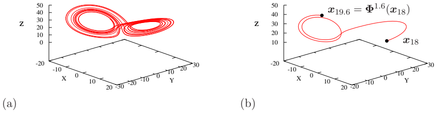
An equilibrium is a fixed point of the flow map for any time, a periodic orbit is a fixed point for its period $T$, and travelling waves and relative periodic orbits become ordinary equilibria and periodic orbits after a symmetry-reducing slice transformation. The paper's central claim is that all of these can be computed by the Jacobian-free Newton–Krylov method applied to $F(x) = \Phi(x) - x = 0$, with Newton steps obtained from GMRES using the finite-difference product in place of the exact Jacobian. Because the method requires only calls to $F$, which is just an existing time stepper, the same code can be pointed at new problems by supplying a “step by $T$” routine. The paper demonstrates this on the Lorenz system, using previously computed periodic orbits as checks, and reports that the same approach has found periodic orbits and travelling waves in a 154755-dimensional pipe-flow simulation.

Load-bearing premise

The load-bearing premise is that the finite-difference approximation of the Jacobian-vector product, with step set so that $(\varepsilon \|\delta x\|)/\|x\|$ is about $10^{-6}$, is accurate enough for GMRES to produce a usable Newton step; if the flow map is insufficiently smooth or the step is badly scaled, the search fails.

Editorial extensions

If this is right

Anyone with a working time stepper can search for equilibria and periodic orbits by plugging that stepper into the supplied template; no Jacobian evaluation or storage is needed.
Travelling waves and relative periodic orbits become ordinary equilibria and periodic orbits under Fourier slicing, so the same solver finds them automatically.
Unknown periods and spatial shifts can be handled by augmenting the unknowns with constraints that keep the Newton update orthogonal to the trajectory and to the shift direction.
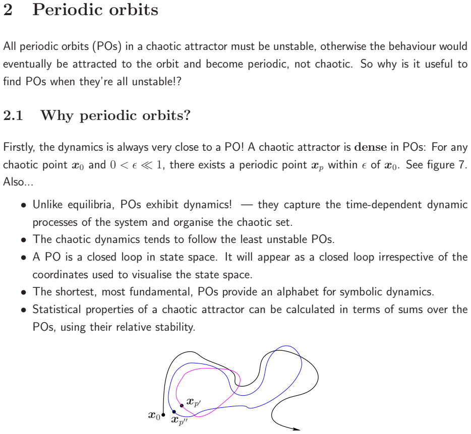
In chaotic systems, the computed periodic orbits can serve as an organising skeleton: near-recurrences shadow them, and their relative stability organises statistical averages.
The method carries over to large systems; the same code was used to find periodic and travelling-wave solutions of a 154755-dimensional pipe-flow model.

Reading between the lines

Editorial extensions of the paper, not claims the author makes directly.

The paper leaves implicit that the practical bottleneck is the initial guess: recurrence plots and symmetry reduction supply candidates, but the automated discovery of good starting points is still open and could be combined with systematic recurrence scanning.
A natural extension not discussed is replacing the finite-difference Jacobian-vector product with complex-step or automatic differentiation where available, which could remove the step-size sensitivity that is the method's load-bearing assumption.
The same fixed-point formulation with augmentations could be aimed at other invariant objects such as heteroclinic connections or unstable manifolds, not just equilibria and periodic orbits.

Share X Bluesky LinkedIn Reddit HN

Editorial analysis

A structured set of objections, weighed in public.

Desk editor's note, referee report, and a circularity audit.

Desk Editor's Note

read the letter

Short version: this is a teaching document, not a research contribution, and it should be judged on that basis. Its genuinely useful piece is the problem-independent Newton-Krylov template with the Lorenz system as a runnable example. The exposition of flow maps, equilibria, periodic orbits, relative orbits, Poincaré sections, slicing, JFNK, the hookstep, and the constraints is accurate and pleasantly direct. I checked Sections 1.3 through 3.4 against the standard references it cites and found no hand-waving where it matters. The Lorenz example reproduces Viswanath's orbits from published initial guesses, which is a real, reproducible demonstration that the code works.

The soft spots are mostly minor. There is no new mathematics, and the paper does not try to hide that; every ingredient is attributed. The finite-difference Jacobian-vector product in (3.8) is presented as a heuristic with a typical epsilon value, with no error analysis and no discussion of when adaptive or event-driven timesteppers will break it. For the target audience—people with smooth, fixed-step timesteppers—this is fine; it is standard Knoll–Keyes practice. A sentence saying 'if convergence stalls, check this epsilon first' would have helped, but its absence is not a flaw in what the paper claims. The blanket statement that chaotic attractors are dense in periodic orbits is a bit breezy, though for the Lorenz system at the standard parameters it is the right intuition and the cited Viswanath computations support it.

On the reader's take: the identified 'weakest assumption' about (3.8) is real but not close to load-bearing for a tutorial of this scope. The method is standard, the example converges, and the paper explicitly frames the template for smooth large systems such as pipe flow, not for every conceivable timestepper.

Who is this for: graduate students and researchers who already have a timestepper and want invariant solutions without writing a solver from scratch. It deserves a serious referee—not because it breaks new ground, but because its pedagogical clarity and reusable code justify the time. I would not cite it in my own papers; I would cite openpipeflow.org and the original sources. But I would hand it to a student without hesitation.

Referee Report

1 major / 6 minor

Summary. The paper is a short pedagogical exposition of how equilibria, periodic orbits, relative periodic orbits, and pre-periodic orbits can be formulated as fixed-point problems for the flow map Phi, and how these fixed points can be computed with the Jacobian-free Newton-Krylov (JFNK) method. The first half defines the flow map, invariant solutions, Poincaré sections, and Fourier slicing for continuous symmetries. The second half develops the Newton-Raphson method, the matrix-free approximation of Jacobian-vector products (Eq. (3.8)), the GMRES iteration, the hookstep trust-region strategy, constraints for the period T and shift l, optional preconditioning, and a practical template code applied to the Lorenz system using known periodic orbits from Viswanath (2003).

Significance. If taken as a tutorial/reference rather than a research contribution, the paper is successful: the mathematical descriptions are accurate and consistent with the cited literature, the practical pitfalls (initial guesses, tolerances, norm choices) are addressed, and the accompanying code (openpipeflow.org) directly illustrates the method on a nontrivial example. The paper does not claim new mathematical results, but it fills a gap by giving a compact, self-contained description of a technique widely used in computational fluid dynamics for finding invariant solutions. The JFNK formulation is standard, and the explanations are clear enough to be used by graduate students.

major comments (1)

[Section 3.2, Eq. (3.8)] The paper states that the method requires little more than calls to an existing time stepping code and suggests a typical finite-difference step with (epsilon ||delta x||)/||x|| = 10^-6. This is reasonable for smooth systems integrated with fixed time steps, but it is not robust for adaptive or event-driven integrators, where the discrete flow map Phi_T may be non-smooth or only piecewise differentiable with respect to the initial condition. The authors should add a sentence cautioning that when adapting the code to an existing timestepper, the user must ensure that the map being differentiated is sufficiently smooth (e.g., by fixing the time step), and should perhaps mention a simple diagnostic (e.g., checking that the finite-difference quotient converges as epsilon is reduced). This does not invalidate the examples in the paper, but it qualifies the claim that little more than calls to a time stepping code is needed.

minor comments (6)

[Section 1.2] The phrase 'we can consider an equilibrium to be a special case of a periodic orbit where T may be arbitrarily chosen' is slightly misleading: for a periodic orbit T is the minimal period, while for an equilibrium any T works; this is a minor wording issue.
[Section 3.2] The GMRES description says 'It is common to start with K1 = b/||b||'; this assumes a zero initial guess for delta x. It would be clearer to state that the initial guess is taken as zero.
[Section 3.5.1] In the expression for ilde{A} = e^A, the scalar '1' should be the identity matrix I.
[Section 4] Typo: 'Z = 27 in call cases' should be 'in all cases'.
[Section 3.4.1] The constraint ang<dot(x)_i, delta x> = 0 requires that dot(x)_i is nonzero; the degenerate case of an equilibrium is not discussed.
[Various] Several typos should be corrected, e.g., 'Kyrlov' in Section 3.5.1, 'pe riodic' in Section 3.4.2, 'section s' in Section 3.4.1, and the missing period after 'is required .' in Section 3.2.

Circularity Check

0 steps flagged · score 0.0 of 10

No significant circularity: the paper is a self-contained exposition of a standard numerical method applied to externally established examples.

full rationale

The paper's derivation chain is F(x) = Phi(x) - x = 0, solved by Newton's method with a Krylov solver whose Jacobian-vector products are approximated by finite differences in equation (3.8). This is a standard, externally established method (Knoll and Keyes, 2004), and the Lorenz system examples are taken from Viswanath (2003), an independent source. The author's own prior works (Willis et al., 2013; Willis et al., 2016; Willis, 2017) are cited as applications or as sources of the openpipeflow code and slicing procedure, not as inputs that already contain the target result. No fitted parameter is renamed as a prediction, no invariant solution is derived from an assumption that already asserts its existence, and no load-bearing uniqueness theorem is imported from the authors' own prior work. The finite-difference approximation in equation (3.8) is an acknowledged practical heuristic, but it is introduced as a standard approximation and its validity is demonstrated by the supplied Lorenz example; it is not a circular step because it does not presuppose the fixed points being sought. The paper is therefore self-contained against external benchmarks and no circularity is present.

Assumptions & free parameters 3 free parameters · 4 assumptions · 0 invented entities

The paper is an exposition of standard numerical methods. It introduces no scientific free parameters or new entities. The only parameters are standard numerical tolerances and step sizes, listed above. It relies on standard mathematical background (Newton's method, GMRES) and domain assumptions about smooth flow maps and density of periodic orbits in chaotic attractors.

free parameters (3)

Finite-difference step factor epsilon = 10^-6 relative
Equation (3.8) uses a finite-difference approximation of the Jacobian-vector product; the step size is chosen by hand as a typical value, not fitted to data.
Newton solution relative tolerance = 10^-8 relative
Section 3.2 states we might seek ||F(x)||/||x|| = O(1e-8) for the Newton solution; a numerical convergence criterion chosen by the user.
GMRES solution relative tolerance = 10^-3 relative
Section 3.2 states a relative error for the GMRES solution of O(1e-3) is likely sufficient; chosen by hand.

assumptions (4)

domain assumption Flow map Phi^t is differentiable and time-stepping gives an accurate evaluation of Phi^T(x).
Required for the finite-difference Jacobian approximation in equation (3.8) and for the residual F(x) = Phi(x) - x to be a smooth function; invoked in Sections 3.2 and 3.4.
standard math Newton's method converges from a sufficiently good initial guess (local convergence theorem).
The entire JFNK iteration in Section 3 relies on the standard local convergence theory of Newton's method; the paper notes convergence is expected if each step is in approximately the correct direction.
standard math GMRES solves the linear system A delta x = b using only matrix-vector products (Krylov subspace method).
Section 3.2 describes GMRES and relies on its property that the solution is in a Krylov subspace; this is standard numerical linear algebra.
domain assumption The attractor is dense in periodic orbits (shadowing), so near-recurrences provide good initial guesses.
Section 2.1 states a chaotic attractor is dense in periodic orbits to justify searching for recurrences; this is a property of hyperbolic (or Lorenz-like) attractors, not general chaotic systems.

how reviews work

0 comments

Cite this review

Pith. "Pith review of Equilibria, periodic orbits and computing them." pith.science (2026). https://pith.science/paper/YVM6FPMO

@misc{pith2026190806730,
  author       = {Pith},
  title        = {Pith review of: Equilibria, periodic orbits and computing them},
  year         = {2026},
  howpublished = {\url{https://pith.science/paper/YVM6FPMO}},
  note         = {Machine review of arXiv:1908.06730}
}

read the original abstract

In this short exposition, we describe equilibria and periodic orbits in terms of the flow map, {\Phi}, and discuss the essentials of the Jacobian-free Newton-Krylov (JFNK) method that can be used to find them. This method requires little more than calls to an existing time stepping code, which {\Phi} can be considered to represent. Fortran90 / MATLAB code is available to try it out for yourself, where, in the template/example the method is applied to the Lorenz system. This code is problem-independent and can be applied to large systems, having initially been developed to find periodic orbits in simulations of pipe flow.

Figures

Figures reproduced from arXiv: 1908.06730 by the authors.

**Figure 2.** Rayleigh–B´enard convection. A pair of convection rolls, w [PITH_FULL_IMAGE:figures/full_fig_p002_2.png] view at source ↗

**Figure 3.** (a) A travelling wave: xt = g(ct) x0. By shifting back, x0 = g(−l) xt = g(−l) Φ t (x). (b) A pre-periodic orbit: x0 = xT , but also x0 = σ xT /2, where σ flips the state about 0. 3 [PITH_FULL_IMAGE:figures/full_fig_p003_3.png] view at source ↗

Figures from the paper (8 more)

**Figure 4.** Figure 4: The shortest periodic orbit of the Lorenz system (1.3) ha [PITH_FULL_IMAGE:figures/full_fig_p004_4.png]

**Figure 5.** Figure 5: (a) A Poincar´e section P, defined by a point x ′ and a normal vector t ′ , is pierced by a periodic orbit at the periodic point xp. (b) The projection of a relative periodic orbit onto a slice Mˆ , is a periodic orbit, xˆt = xˆt+T . The whole orbit is projected onto M…

**Figure 6.** Figure 6: (a) Fourier slicing: A state x is mapped onto the (a1, a2)-plane, where all shifted versions of x map onto a circle. All versions are reduced to the single copy xˆ = g(−(θ/2π)L) x. (b) A travelling wave is reduced to an equilibrium. lt is automatically determined by th…

**Figure 7.** Figure 7: ‘Shadowing’ of a chaotic trajectory by periodic orbits. By [PITH_FULL_IMAGE:figures/full_fig_p006_7.png]

**Figure 8.** Figure 8: A few of the shortest periodic orbits of the Lorenz syste [PITH_FULL_IMAGE:figures/full_fig_p007_8.png]

**Figure 9.** Figure 9: (left) Visualisation of pipe flow with slow streaks (blue) and vortices (yellow). (right) Periodic orbits of pipe flow. Inset is view from bottom left side of box. (Reproduction of figure 4 of Willis et al., 2016) 7 [PITH_FULL_IMAGE:figures/full_fig_p007_9.png]

**Figure 10.** Figure 10: is an example for pipe flow. We then look for local minima in the plot that provide candidate recurrent points, xp ≈ xt−∆t and T ≈ ∆t. The normalisation factor might be chosen to depend on both ||xt || and ||xt−∆t ||, or might not be necessary at all. A complication i…

**Figure 11.** Figure 11: Hookstep versus ‘damped’/line-search step of the same [PITH_FULL_IMAGE:figures/full_fig_p011_11.png]

Discussion (0). Continue with ORCID to comment.

Forward citations

Cited by 2 Pith papers

Reviewed papers in the Pith corpus that reference this work. Sorted by Pith novelty score. Full citation record

Effects of symmetry and hydrodynamics on the cohesion of groups of swimmers
physics.flu-dyn 2025-05 conditional novelty 6.0 of 10

Using a 3D far-field potential-flow model, the authors show that passive hydrodynamic interactions can keep small swimmer groups together, while large groups break into smaller cohesive subgroups and the circular hydr...
Numerical solutions of fixed points in two-dimensional Kuramoto-Sivashinsky equation expedited by reinforcement learning
cs.LG 2024-12 conditional novelty 5.0 of 10

A DRL-assisted Jacobian-Free Newton-Krylov method finds 303 fixed points of the 2D Kuramoto-Sivashinsky equation on a 20x20 periodic domain.

Reference graph

Works this paper leans on

10 extracted references · 10 canonical work pages · cited by 2 Pith papers

[1]

Budanur, N. B., P. Cvitanovi\'c, R. L. Davidchack, and E. Siminos (2015). Reduction of the SO(2) symmetry for spatially extended dynamical systems. Phys. Rev. Lett.\/ 114 , 084102

work page 2015
[2]

Cvitanovi \'c , P. and J. F. Gibson (2010). Geometry of turbulence in wall-bounded shear flows: Periodic orbits. Phys. Scr. T\/ 142 , 014007

work page 2010
[3]

Dennis, J. and R. Schnabel (1996). Numerical Methods for Unconstrained Optimization and Nonlinear Equations . SIAM

work page 1996
[4]

Knoll, D. A. and D. E. Keyes (2004). Jacobian-free N ewton-- K rylov methods: a survey of approaches and applications. Journal of Computational Physics\/ 193\/ (2), 357--397

work page 2004
[5]

Lorenz, E. N. (1963). Deterministic nonperiodic flow. J. Atmos. Sci.\/ 20 , 130--141

work page 1963
[6]

Viswanath, D. (2003). Symbolic dynamics and periodic orbits of the Lorenz attractor. Nonlinearity\/ 16 , 1035--1056

work page 2003
[7]

Viswanath, D. (2007). Recurrent motions within plane Couette turbulence. J. Fluid Mech.\/ 580 , 339--358

work page 2007
[8]

Willis, A. (2017). The O penpipeflow N avier-- S tokes solver. SoftwareX\/ 6 , 124--127

work page 2017

Show all 10 references

[9]

Willis, A. P., P. Cvitanovi \'c , and M. Avila (2013). Revealing the state space of turbulent pipe flow by symmetry reduction. J. Fluid Mech.\/ 721 , 514--540

2013
[10]

Willis, A. P., K. Y. Short, and P. Cvitanovi \'c (2016). Symmetry reduction in high dimensions, illustrated in a turbulent pipe. Phys. Rev. E\/ 93 , 022204

2016

Pith tools

Reviewed August 14, 2026 · model on record in the stance chip above.

[1] [1]

Budanur, N. B., P. Cvitanovi\'c, R. L. Davidchack, and E. Siminos (2015). Reduction of the SO(2) symmetry for spatially extended dynamical systems. Phys. Rev. Lett.\/ 114 , 084102

work page 2015

[2] [2]

Cvitanovi \'c , P. and J. F. Gibson (2010). Geometry of turbulence in wall-bounded shear flows: Periodic orbits. Phys. Scr. T\/ 142 , 014007

work page 2010

[3] [3]

Dennis, J. and R. Schnabel (1996). Numerical Methods for Unconstrained Optimization and Nonlinear Equations . SIAM

work page 1996

[4] [4]

Knoll, D. A. and D. E. Keyes (2004). Jacobian-free N ewton-- K rylov methods: a survey of approaches and applications. Journal of Computational Physics\/ 193\/ (2), 357--397

work page 2004

[5] [5]

Lorenz, E. N. (1963). Deterministic nonperiodic flow. J. Atmos. Sci.\/ 20 , 130--141

work page 1963

[6] [6]

Viswanath, D. (2003). Symbolic dynamics and periodic orbits of the Lorenz attractor. Nonlinearity\/ 16 , 1035--1056

work page 2003

[7] [7]

Viswanath, D. (2007). Recurrent motions within plane Couette turbulence. J. Fluid Mech.\/ 580 , 339--358

work page 2007

[8] [8]

Willis, A. (2017). The O penpipeflow N avier-- S tokes solver. SoftwareX\/ 6 , 124--127

work page 2017