REVIEW 3 major objections 4 minor 1 cited by
Building Interpretable Climate Emulators for Economics
T0 review · 3 major / 4 minor · reviewed 2026-08-12 · deepseek-v4-flash
Pith's one-line read Representing deforestation-driven loss of land carbon storage raises the optimal social cost of carbon by up to 17 US$ per tonne of CO2 within a DICE-2016-style model.
desk verdict A transparent, reproducible emulator framework whose static-box calibration deserves publication, but whose headline land-use SCC results rest on an acknowledged, uncalibrated r=1 assumption and should be treated as a scenario until sensitivity analysis is added. read the letter →
The pith
A machine-rendered reading of the paper's core claim, the machinery that carries it, and where it could break.
The reading
What carries the argument
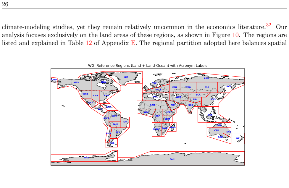
The central object is the generalized linear multi-reservoir carbon-cycle operator A (a mass-conserving, equilibrium-constrained box model) with a time-dependent land-biosphere equilibrium mass. The decisive element is the update $\tilde{m}^L_{t+1} = \tilde{m}^L_t - r\, e^L_t$ with $r=1$, which shrinks the land reservoir's carbon holding capacity in lockstep with land-use emissions, forcing a larger share of emitted carbon to remain in the atmosphere. Calibration fits the operator's fluxes and equilibrium masses to the multi-model mean of the 100 GtC pulse-decay benchmark, with penalty terms for dynamic timescales, equilibrium masses, and ocean-to-land uptake ratios; a second layer rescales eigenvalues to emulate fast and slow extremes. For spatial downscaling, the workhorse is the linear pattern-scaling relation $\Delta T^z = \Delta T^{AT}\, \beta^z$ combined with an observational climatology to obtain absolute regional temperatures.
What would settle it
Estimate r directly from data: compare cumulative land-use emissions against observed losses of global vegetation and soil carbon stocks; an r of, say, 0.3 instead of 1 would cut the 0.2 °C and 17 USD effects proportionally. Equivalently, drive the 4PR-X emulator with historical land-use emissions from 1850 onward and check whether the simulated atmospheric CO2 trajectory remains within the observed ice-core and Mauna Loa record; a systematic divergence would falsify the one-for-one sink-loss mechanism.
Extended reading notes
Core claim
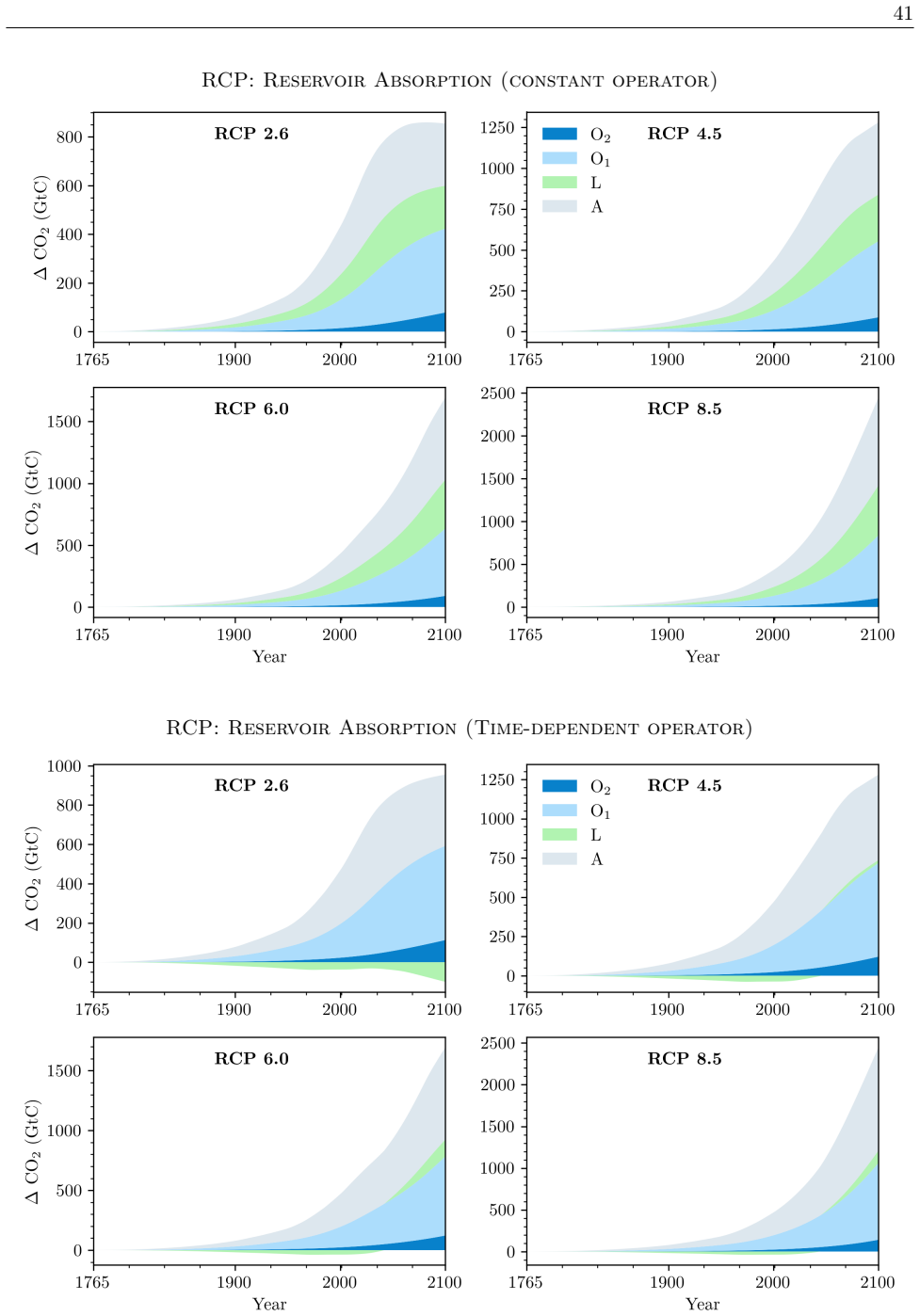
Representing the land biosphere as a dynamic reservoir whose equilibrium carbon mass falls in proportion to land-use emissions (the 4PR-X model) materially alters the climate-economy outcome relative to the static three- and four-box emulators. Under business-as-usual and optimal mitigation, the 4PR-X emulator projects atmospheric carbon about 6% higher (~80 GtC) and global-mean temperature about 0.2 °C higher by 2100, raising the optimal social cost of carbon by 11.9–13.9% in 2020–2050 (up to 17 USD per tCO2). The fourth reservoir alone does nothing: the static 4PR model reproduces 3SR behavior almost exactly. The result is driven by an explicit mechanism: each ton of deforestation carbon emits CO2 and simultaneously removes one ton of permanent land storage capacity, so more carbon remains airborne; the paper explicitly flags that the one-to-one relationship (r=1) is an assumption.
Load-bearing premise
The whole policy effect rests on the assumption that each ton of carbon emitted through land-use change permanently removes one ton of carbon storage capacity from the land biosphere in the emulator; if the true loss is smaller or delayed, the extra warming and higher carbon price shrink accordingly.
Editorial extensions
If this is right
- DICE-type integrated assessment models that omit deforestation-driven loss of land carbon storage underestimate future atmospheric carbon, warming, and the optimal carbon price needed to offset them.
- Policy evaluations of carbon capture and storage are overly optimistic unless land-use change is controlled: the 4PR-X model shows that CCS alone leaves temperatures about 7% higher in 2100 if deforestation continues.
- Adding a static land-biosphere box to a three-box carbon cycle changes atmospheric carbon, temperature, and SCC by negligible amounts; the improvement comes only when the land reservoir's capacity responds to land-use emissions.
- Pattern-scaling choices carry real economic weight: anchoring regional warming to different present-day climatologies can shift 2100 regional mean temperatures by up to roughly 3 °C, which can flip a region from a relative winner to a relative loser in a hump-shaped damage function.
- Emulator calibration to present-day rather than pre-industrial conditions changes the trajectory but preserves the qualitative ordering, with present-day initialization yielding higher accumulation and higher SCC.
Reading between the lines
- If the r=1 assumption is relaxed to a value calibrated against observed biomass-loss data, the SCC uplift would likely shrink but remain positive for any r>0; the paper's headline numbers should be read as an upper-bound estimate of the deforestation feedback.
- The same shrinking-sink mechanism could be ported to other compact climate models used for policy (impulse-response or reduced-complexity emulators), where land-use emissions are currently treated purely as an atmospheric source rather than as a reduction in future uptake capacity.
- A testable extension is to couple the dynamic land reservoir with a simple carbon-cycle non-linearity such as saturating CO2 fertilization; under high emissions that non-linearity would reinforce the 4PR-X effect, making the 0.2 °C a lower bound at high concentration.
- The pattern-scaling uncertainty decomposition suggests that spatial integrated assessment models should treat the warming pattern and the baseline climatology as separate, hedgeable uncertainty sources rather than pooling them into one damage-function risk.
Signed reviews
Editorial analysis
A structured set of objections, weighed in public.
Referee Report
Summary. The paper develops an open-source framework for building interpretable, physically constrained linear box-model carbon-cycle emulators for use in economic integrated assessment models. Three emulators are constructed and compared within a DICE-2016-style model: a three-reservoir model (3SR), a four-reservoir model with a static land box (4PR), and a four-reservoir model with a dynamic land capacity that declines with land-use emissions (4PR-X). The authors find that 3SR and 4PR give nearly identical results, while 4PR-X produces substantially higher atmospheric carbon, temperature, and social cost of carbon by 2100. A second contribution propagates global-mean temperature projections to regional scales via pattern scaling using the Lynch et al. (2017) CMIP5 pattern library, and illustrates how choices of warming pattern and observational baseline affect regional damage estimates.
Significance. If the quantitative claims are upheld, the paper makes a useful methodological contribution: it provides a transparent, reproducible, and physically interpretable alternative to black-box climate emulators, with code publicly available and validation against the Joos et al. (2013) pulse-decay benchmark as well as ZECMIP and RCP-style tests. The finding that a static land box hardly changes DICE outcomes while a dynamic land-capacity representation materially increases warming and SCC is a policy-relevant result for the IAM community. The pattern-scaling module is a useful plug-and-play addition, clearly separating emulator, pattern, and baseline uncertainties. However, the headline quantitative results for 4PR-X are driven by an uncalibrated parameter, and the accuracy claims in the abstract and Section 3.1.4 are contradicted by the paper's own Appendix A.2, so the current version does not yet establish the magnitude of the claimed effects.
major comments (3)
- [Section 2.1, Eq. (7); Tables 3-5] The central quantitative result—approximately 80 GtC higher atmospheric carbon, 0.2°C extra warming, and 12–14% higher SCC in 4PR-X relative to the static models—is generated entirely by the assumption r=1 in Eq. (7), which sets the decline in equilibrium land-biosphere capacity equal to one-for-one land-use emissions. The paper explicitly acknowledges in Section 2.1 that 'a one-to-one correspondence ... may not be guaranteed' and that 'r could be different from 1,' yet no sensitivity analysis is reported. Because all differences between 4PR-X and the static models scale with r, the quantitative headline is conditional on this uncalibrated assumption. I request a sensitivity analysis over a plausible range of r (e.g., 0.25, 0.5, 0.75, 1) for the BAU and optimal mitigation runs, and reporting of how the 2100 atmospheric carbon, temperature, and SCC differences respond. If results shrink substantially for lower r, the abstract and conclusions should be reframed as qualitative.
- [Abstract; Section 3.1.4; Appendix A.2, Figure 21] The abstract and Section 3.1.4 claim that the three- and four-box emulators 'reproduce the historical and long-run evolution of atmospheric CO2 and global temperature to within about 5% and 3%, respectively.' This is contradicted by Appendix A.2, which states that the PI-calibrated 3SR and 4PR models 'systematically underestimate atmospheric CO2' under RCP scenarios, and Figure 21 shows these models falling well below the CMIP5 RCP concentration trajectories. The 5%/3% accuracy figure appears to refer to the atmospheric-pulse-decay fit error (Figures 15 and 24), not to historical or scenario concentration accuracy. Please clarify precisely which metric the accuracy claim refers to, and either qualify or remove the broad claim.
- [Appendix A.2, Table 11, Section 4.2] The 4PR-X model's equilibrium land-biosphere mass in 2015 is 258 GtC (Table 11), far below the Ciais et al. (2014) active land-pool estimate of ~550 GtC cited in Section 3.1.1, and below the 4PR value of 387 GtC. The paper acknowledges this in Section 4.2, noting that the low 2015 land content is 'slightly outside the estimated range.' This implausibly low land pool is a direct consequence of applying r=1 cumulatively to historical land-use emissions, and it contributes to the elevated atmospheric burden in 4PR-X. The paper should discuss whether this initial-condition distortion unduly inflates the projected differences, and whether an r<1 calibration or a cap on the equilibrium-mass decline would yield more realistic land-pool trajectories.
minor comments (4)
- [Table 6] The table header uses '3PR' as the column label, which is inconsistent with the '3SR' nomenclature used throughout the paper.
- [Appendix A.1.1, Figure 16 caption] The caption states that 'the q1 penalty function enforces an approximately equal mass of carbon absorption between the oceans and the land biosphere,' but this is the role of the q3 penalty (reservoir absorption ratios), not q1 (dynamic timescales). Please correct the reference.
- [Section 5.2, Table 7] The comparison of anchoring choices in Table 7 conflates two differences: the baseline period (1961-1990 for model climatologies vs 1991-2020 for ERA5) and the use of model versus observed climatology. The statement that the anchor choice can shift 2100 regional means by 'up to 2.5-3°C' should be decomposed into these two effects, since the baseline-period difference alone can explain part of the spread.
- [Figure 12 text] There is a typo in the paragraph above Figure 12: 'model undertainty' should be 'model uncertainty.'
Circularity Check
No significant circularity: the 4PR-X results are conditional on an explicitly flagged r=1 assumption, not on a fitted parameter renamed as a prediction or on a load-bearing self-citation chain.
full rationale
The central quantitative claim (about 80 GtC, 0.2°C, and 12–14% SCC differences) is generated by the 4PR-X operator in Eq. (34) with the land equilibrium mass evolving according to Eq. (7) at r=1. This is an explicit structural assumption, and the paper flags its uncertainty: Section 2.1 states, 'In our simplified setting we adopt a one-to-one correspondence (r = 1)... The proportionality factor r could be different from 1.' The paper never fits r to the atmospheric data whose response it then reports; the pulse-decay calibration in Section 3.1.1 constrains the transfer coefficients and equilibrium masses under a fixed land equilibrium mass, and the q3 penalty targets a pulse-absorption ratio, not land-use-driven capacity loss. The 4PR-X-versus-static divergence is therefore a conditional scenario output, not a disguised refit of the same target. The direction of the effect (a shrinking land sink leaves more carbon in the atmosphere) is indeed built into Eqs. (7) and (34), but the paper presents this as the modeled mechanism and explicitly cautions that r may differ from 1, so the headline numbers are not presented as an independently measured empirical prediction. External anchors do exist for the parts of the framework that are claimed as predictions: the pulse-decay calibration uses the external Joos et al. (2013) multi-model mean with out-of-sample validation for t>250 (Appendix A.1.1), the zero-emissions commitment experiments are checked against MacDougall et al. (2020), and the pattern-scaling analysis uses the external CMIP5 pattern library of Lynch et al. (2017). Self-citations to Folini et al. (2024) supply the temperature module and calibration-data justification, but they are not load-bearing for the land-use channel that drives the paper's main new results. Accordingly, no circular step meets the required standard of exhibiting a specific reduction of a claimed prediction to its own fitted inputs or to a self-citation chain.
Assumptions & free parameters
free parameters (3)
- r (land-use emission to equilibrium-mass conversion factor) =
1 (assumed, not fitted)
- Penalty weights ρ1, ρ2, ρ3 =
1e-2, 1e-4, 1e-4 (3SR: ρ3=0)
- Extreme scaling factors c_mu+ and c_mu- =
3SR: 0.4746 and 2.4559; 4PR: 0.4701 and 2.4074
assumptions (5)
- domain assumption Linear box model with mass conservation and eigenvalues in (-1,0]
- domain assumption Two-layer energy balance temperature model with logarithmic CO2 forcing
- domain assumption Pattern scaling linearity with stationary βz
- domain assumption Inverted-U regional damage function
- ad hoc to paper r=1 one-for-one land capacity reduction
Cite this review
Pith. "Pith review of Building Interpretable Climate Emulators for Economics." pith.science (2026). https://pith.science/paper/Z2YW3IQN
@misc{pith2026241110768,
  author       = {Pith},
  title        = {Pith review of: Building Interpretable Climate Emulators for Economics},
  year         = {2026},
  howpublished = {\url{https://pith.science/paper/Z2YW3IQN}},
  note         = {Machine review of arXiv:2411.10768}
}
read the original abstract
We introduce a framework for developing efficient and interpretable climate emulators (CEs) for economic models of climate change. The paper makes two main contributions. First, we propose a general framework for constructing carbon-cycle emulators (CCEs) for macroeconomic models. The framework is implemented as a generalized linear multi-reservoir (box) model that conserves key physical quantities and can be customized for specific applications. We consider three versions of the CCE, which we evaluate within a simple representative agent economic model: (i) a three-box setting comparable to DICE-2016, (ii) a four-box extension, and (iii) a four-box version that explicitly captures land-use change. While the three-box model reproduces benchmark results well and the fourth reservoir adds little, incorporating the impact of land-use change on the carbon storage capacity of the terrestrial biosphere substantially alters atmospheric carbon stocks, temperature trajectories, and the optimal mitigation path. Second, we investigate pattern-scaling techniques that transform global-mean temperature projections from CEs into spatially heterogeneous warming fields. We show how regional baseline climates, non-uniform warming, and the associated uncertainties propagate into economic damages.
Figures


Figures from the paper (29 more)






Forward citations
Cited by 1 Pith paper
-
Using Machine Learning to Compute Constrained Optimal Carbon Tax Rules
A Pareto-improving linear tax on cumulative emissions with optimal transfers yields a 0.42% aggregate welfare gain in a stochastic OLG climate model, and more complex taxes add only 0.03 percentage points.
Reference graph
Works this paper leans on
-
[1]
Arora , Vivek K., Anna Katavouta , Richard G. Williams , Chris D. Jones , Victor Brovkin , Pierre Friedlingstein , J \"o rg Schwinger , Laurent Bopp , Olivier Boucher , Patricia Cadule , Matthew A. Chamberlain , James R. Christian , Christine Delire , Rosie A. Fisher , Tomohiro Hajima , Tatiana Ilyina , Emilie Joetzjer , Michio Kawamiya , Charles D. Koven...
work page 2020
-
[2]
str \"o m, Karl Johan and Richard Murray. 2021. Feedback systems: an introduction for scientists and engineers. Princeton university press
work page 2021
-
[3]
Azinovic, Marlon, Luca Gaegauf, and Simon Scheidegger. 2022. Deep equilibrium nets. International Economic Review 63 (4):1471--1525
work page 2022
-
[4]
Beusch, L., L. Gudmundsson, and S. I. Seneviratne. 2020. Emulating Earth system model temperatures with MESMER: F rom global mean temperature trajectories to grid-point-level realizations on land. Earth System Dynamics 11 (1):139--159
work page 2020
-
[5]
Bilbao , Roberto A. F., Jonathan M. Gregory , and Nathaelle Bouttes . 2015. Analysis of the regional pattern of sea level change due to ocean dynamics and density change for 1993-2099 in observations and CMIP5 AOGCMs . Climate Dynamics 45 (9-10):2647--2666
work page 2015
-
[6]
Cai, Yongyang and Thomas Lontzek. 2019. The social cost of carbon with economic and climate risks . Journal of Political Economy 127 (6):2684--2734
work page 2019
-
[7]
Page Kyle, Pralit Patel, Pralit Patel, Leon Clarke, Leon E
Calvin, Katherine, Katherine Calvin, Marshall Wise, Marshall Wise, Page Kyle, Page Kyle, G. Page Kyle, Pralit Patel, Pralit Patel, Leon Clarke, Leon E. Clarke, James A. Edmonds, and James A. Edmonds. 2014. Trade-offs of different land and bioenergy policies on the path to achieving climate targets. Climatic Change
work page 2014
- [8]
Show all 65 references
-
[9]
Cruz, Jos \'e -Luis and Esteban Rossi-Hansberg. 2024. The economic geography of global warming . Review of Economic Studies 91 (2):899--939
2024
-
[10]
Desmet, Klaus and Esteban Rossi-Hansberg. 2024. Climate change economics over time and space. Annual Review of Economics 16:271--304
2024
-
[11]
Dietz, Simon. 2024. Chapter 1 - Introduction to integrated assessment modeling of climate change. North-Holland, 1--51. ://www.sciencedirect.com/science/article/pii/S3050729424000023
2024
-
[12]
Dietz, Simon and Frank Venmans. 2019. Cumulative carbon emissions and economic policy: In search of general principles . Journal of Environmental Economics and Management 96:108--129. ://doi.org/10.1016/j.jeem.2019.04.003
2019 doi
-
[13]
Doelman, Jonathan Doelman, Jonathan C
Doelman, Jonathan C., Jonathan C. Doelman, Jonathan Doelman, Jonathan C. Doelman, Jonathan C. Doelman, Elke Stehfest, Elke Stehfest, Elke Stehfest, Detlef P. van Vuuren, Detlef P. van Vuuren, Andrzej Tabeau, Andrzej Tabeau, Andries F. Hof, Andries F. Hof, Maarten C. Braakhekke...
2020
-
[14]
Shiklomanov , Steven J
Dorheim , Kalyn, Skylar Gering , Robert Gieseke , Corinne Hartin , Leeya Pressburger , Alexey N. Shiklomanov , Steven J. Smith , Claudia Tebaldi , Dawn L. Woodard , and Ben Bond-Lamberty . 2024. Hector V3.2.0: Functionality And Performance Of A Reduced-Complexity Climate Model...
2024
-
[15]
Gillingham, and Simon Scheidegger
Fernández-Villaverde, Jesús, Kenneth T. Gillingham, and Simon Scheidegger. 2025. Climate Change Through the Lens of Macroeconomic Modeling. Annual Review of Economics ://www.annualreviews.org/content/journals/10.1146/annurev-economics-091124-045357
2025 doi
-
[16]
Folini, Doris, Aleksandra Friedl, Felix K \"u bler, and Simon Scheidegger. 2024. The climate in climate economics. Review of Economic Studies :rdae011
2024
-
[17]
Friedl, Aleksandra, Felix K \"u bler, Simon Scheidegger, and Takafumi Usui. 2023. Deep uncertainty quantification: With an application to integrated assessment models. Working paper, University of Lausanne
2023
-
[18]
Lamb , Max W
Fuss , Sabine, William F. Lamb , Max W. Callaghan , J \'e r \^o me Hilaire , Felix Creutzig , Thorben Amann , Tim Beringer , Wagner de Oliveira Garcia , Jens Hartmann , Tarun Khanna , Gunnar Luderer , Gregory F. Nemet , Joeri Rogelj , Pete Smith , Jos \'e Luis Vicente Vicente ...
2018
-
[19]
Gasser , Thomas, Philippe Ciais , Olivier Boucher , Yann Quilcaille , Maxime Tortora , Laurent Bopp , and Didier Hauglustaine . 2017. The compact Earth system model OSCAR v2.2: description and first results . Geoscientific Model Development 10 (1):271--319
2017
-
[20]
Saint-Martin, G
Geoffroy, Olivier, D. Saint-Martin, G. Bellon, A. Voldoire, D. J.L. Olivi \' e , and S. Tyt \' e ca. 2013 a . Transient climate response in a two-layer energy-balance model. Part II: Representation of the efficacy of deep-ocean heat uptake and validation for CMIP5 AOGCMs . Jou...
2013
-
[21]
Saint-martin, D
Geoffroy, Olivier, D. Saint-martin, D. J.L. Olivi \' e , A. Voldoire, G. Bellon, and S. Tyt \' e ca. 2013 b . Transient climate response in a two-layer energy-balance model. Part I: Analytical solution and parameter calibration using CMIP5 AOGCM experiments . Journal of Climat...
2013
-
[22]
Pierrehumbert , Joshua W
Glotter , Michael J., Raymond T. Pierrehumbert , Joshua W. Elliott , Nathan J. Matteson , and Elisabeth J. Moyer . 2014. A simple carbon cycle representation for economic and policy analyses . Climatic Change 126 (3-4):319--335
2014
-
[23]
Hassler, John, Per Krusell, and Conny Olovsson. 2023. Climate policy in the wide world. Manuscript
2023
-
[24]
Hernanz, Alfonso, Carlos Correa, Juan Andrés García-Valero , Marta Domínguez, Esteban Rodríguez-Guisado, and Ernesto Rodríguez-Camino. 2023. pyClim-SDM: Service for generation of statistically downscaled climate change projections supporting national adaptation strategies. Cli...
2023
-
[25]
Hersbach , Hans, Bill Bell , Paul Berrisford , Shoji Hirahara , Andr \'a s Hor \'a nyi , Joaqu \' n Mu \ n oz-Sabater , Julien Nicolas , Carole Peubey , Raluca Radu , Dinand Schepers , Adrian Simmons , Cornel Soci , Saleh Abdalla , Xavier Abellan , Gianpaolo Balsamo , Peter Be...
2020
-
[26]
Voss , K
Hooss , G., R. Voss , K. Hasselmann , E. Maier-Reimer , and F. Joos . 2001. A nonlinear impulse response model of the coupled carbon cycle-climate system (NICCS) . Climate Dynamics 18 (3-4):189--202
2001
-
[27]
Houghton, John Theodore, G. J. Jenkins, and J. J. Ephraums, editors. 1990. Climate Change: The IPCC Scientific Assessment. Cambridge University Press. ://www.cambridge.org/eng/academic/subjects/earth-and-environmental-science/climatology-and-climate-change/climate-change-ipcc-...
1990
-
[28]
Hurtt, G. C., L. P. Chini, S. Frolking, R. A. Betts, J. Feddema, G. Fischer, J. P. Fisk, K. Hibbard, R. A. Houghton, A. Janetos, C. D. Jones, G. Kindermann, T. Kinoshita, Kees Klein Goldewijk, K. Riahi, E. Shevliakova, S. Smith, E. Stehfest, A. Thomson, P. Thornton, D. P. van ...
2011
-
[29]
Iturbide, M., J. M. Guti\'errez, L. M. Alves, J. Bedia, R. Cerezo-Mota, E. Cimadevilla, A. S. Cofi\ no, A. Di Luca, S. H. Faria, I. V. Gorodetskaya, M. Hauser, S. Herrera, K. Hennessy, H. T. Hewitt, R. G. Jones, S. Krakovska, R. Manzanas, D. Mart\' nez-Castro, G. T. Narisma, I...
2020
-
[30]
Jenkins , Stuart, Michelle Cain , Pierre Friedlingstein , Nathan Gillett , Tristram Walsh , and Myles R. Allen . 2021. Quantifying non-CO2 contributions to remaining carbon budgets . npj Climate and Atmospheric Science 4 (1):47
2021
-
[31]
Jones , P. D., M. New , D. E. Parker , S. Martin , and I. G. Rigor . 1999. Surface air temperature and its changes over the past 150 years . Reviews of Geophysics 37 (2):173--199
1999
-
[32]
Joos, Fortunat, Raphael Roth, Jan S Fuglestvedt, Glen P Peters, Ian G Enting, W von Bloh, Victor Brovkin, Eleanor J Burke, Michael Eby, Neil R Edwards et al. 2013. Carbon dioxide and climate impulse response functions for the computation of greenhouse gas metrics: a multi-mode...
2013
-
[33]
Kotlikoff, Laurence, Felix Kubler, Andrey Polbin, and Simon Scheidegger. 2024. Can today’s and tomorrow’s world uniformly gain from carbon taxation? European Economic Review 168:104819
2024
-
[34]
Kravitz, Ben, Cary Lynch, Corinne Hartin, and Ben Bond-Lamberty . 2017. Exploring precipitation pattern scaling methodologies and robustness among CMIP5 models. Geoscientific Model Development 10 (5):1889--1902
2017
-
[35]
Smith, Anthony A
Krusell, Per and Jr. Smith, Anthony A. 2022. Climate change around the world. Working Paper 30338, National Bureau of Economic Research
2022
-
[36]
Smith , John Lynch , Michelle Cain , Tristram Walsh , Bill Wu , Junichi Tsutsui , and Myles R
Leach , Nicholas J., Stuart Jenkins , Zebedee Nicholls , Christopher J. Smith , John Lynch , Michelle Cain , Tristram Walsh , Bill Wu , Junichi Tsutsui , and Myles R. Allen . 2021. FaIRv2.0.0: a generalized impulse response model for climate uncertainty and future scenario exp...
2021
-
[37]
Lenton, Timothy M, Hermann Held, Elmar Kriegler, Jim W Hall, Wolfgang Lucht, Stefan Rahmstorf, and Hans Joachim Schellnhuber. 2008. Tipping elements in the Earth's climate system. Proceedings of the National Academy of Sciences 105 (6):1786--1793
2008
-
[38]
Jarvis , and David T
Li , Sile, Andrew J. Jarvis , and David T. Leedal . 2009. Are response function representations of the global carbon cycle ever interpretable? Tellus Series B Chemical and Physical Meteorology B 61 (2):361--371
2009
-
[39]
Lynch, Cary, Corinne Hartin, Ben Bond-Lamberty, and Ben Kravitz. 2017. An open-Access CMIP5 pattern library for temperature and precipitation: Description and methodology . Earth System Science Data 9 (1):281--292
2017
-
[40]
olicher, C. D. Jones, J. Rogelj, H. D. Matthews, K. Zickfeld, V. K. Arora, N. J. Barrett, V. Brovkin, F. A. Burger, M. Eby, A. V. Eliseev, T. Hajima, P. B. Holden, A. Jeltsch-Th\
MacDougall, A. H., T. L. Fr\"olicher, C. D. Jones, J. Rogelj, H. D. Matthews, K. Zickfeld, V. K. Arora, N. J. Barrett, V. Brovkin, F. A. Burger, M. Eby, A. V. Eliseev, T. Hajima, P. B. Holden, A. Jeltsch-Th\"ommes, C. Koven, N. Mengis, L. Menviel, M. Michou, I. I. Mokhov, A. O...
2020
-
[41]
Mathison, C. T., E. Burke, E. Kovacs, G. Munday, C. Huntingford, C. Jones, C. Smith, N. Steinert, A. Wiltshire, L. Gohar, and R. Varney. 2024. A rapid application emissions-to-impacts tool for scenario assessment: Probabilistic regional impacts from model patterns and emission...
2024
-
[42]
Burke , Gregory Munday , Chris D
Mathison , Camilla, Eleanor J. Burke , Gregory Munday , Chris D. Jones , Chris J. Smith , Norman J. Steinert , Andy J. Wiltshire , Chris Huntingford , Eszter Kovacs , Laila K. Gohar , Rebecca M. Varney , and Douglas McNeall . 2025. A Rapid-Application Emissions-To-Impacts Tool...
2025
-
[43]
Tanioka, and J
Matsumoto, K., T. Tanioka, and J. Zahn. 2021. MESMO 3: Flexible phytoplankton stoichiometry and refractory dissolved organic matter. Geoscientific Model Development 14 (4):2265--2288
2021
-
[44]
Mauritsen , Thorsten, Bjorn Stevens , Erich Roeckner , Traute Crueger , Monika Esch , Marco Giorgetta , Helmuth Haak , Johann Jungclaus , Daniel Klocke , Daniela Matei , Uwe Mikolajewicz , Dirk Notz , Robert Pincus , Hauke Schmidt , and Lorenzo Tomassini . 2012. Tuning the cli...
2012
-
[45]
Meinshausen , Malte, S. J. Smith , K. Calvin , J. S. Daniel , M. L. T. Kainuma , J. F. Lamarque , K. Matsumoto , S. A. Montzka , S. C. B. Raper , K. Riahi , A. Thomson , G. J. M. Velders , and D. P. P. van Vuuren . 2011. The RCP greenhouse gas concentrations and their extensio...
2011
-
[46]
Melnikova , Irina, Philippe Ciais , Olivier Boucher , and Katsumasa Tanaka . 2023. Assessing carbon cycle projections from complex and simple models under SSP scenarios . Climatic Change 176 (12):168
2023
-
[47]
Lamb , Max W
Minx , Jan C., William F. Lamb , Max W. Callaghan , Sabine Fuss , J \'e r \^o me Hilaire , Felix Creutzig , Thorben Amann , Tim Beringer , Wagner de Oliveira Garcia , Jens Hartmann , Tarun Khanna , Dominic Lenzi , Gunnar Luderer , Gregory F. Nemet , Joeri Rogelj , Pete Smith ,...
2018
-
[48]
Munday, Gregory, Chris Jones, Norman Steinert, Camilla Mathison, Eleanor Burke, Chris Smith, Chris Huntingford, Rebecca Varney, and Andy Wiltshire. 2025. Risks of unavoidable impacts on forests at 1.5 °C with and without overshoot. Nature Climate Change :1--6
2025
-
[49]
Callaghan , Felix Creutzig , Sabine Fuss , Jens Hartmann , J \'e r \^o me Hilaire , William F
Nemet , Gregory F., Max W. Callaghan , Felix Creutzig , Sabine Fuss , Jens Hartmann , J \'e r \^o me Hilaire , William F. Lamb , Jan C. Minx , Sophia Rogers , and Pete Smith . 2018. Negative emissions Part 3: Innovation and upscaling . Environmental Research Letters 13 (6):063003
2018
-
[50]
Meinshausen , J
Nicholls , Z., M. Meinshausen , J. Lewis , M. Rojas Corradi , K. Dorheim , T. Gasser , R. Gieseke , A. P. Hope , N. J. Leach , L. A. McBride , Y. Quilcaille , J. Rogelj , R. J. Salawitch , B. H. Samset , M. Sandstad , A. Shiklomanov , R. B. Skeie , C. J. Smith , S. J. Smith , ...
2021
-
[51]
Nocedal, Jorge and Stephen J. Wright. 2006. Numerical optimization. Springer series in operations research and financial engineering. New York, NY: Springer, 2. ed. ed. ://gso.gbv.de/DB=2.1/CMD?ACT=SRCHA&SRT=YOP&IKT=1016&TRM=ppn+502988711&sourceid=fbw_bibsonomy
2006
-
[52]
Nordhaus, William D. 2017. Revisiting the Social Cost of Carbon. Proceedings of the National Academy of Sciences 114 (7):1518 LP -- 1523
2017
-
[53]
Pfahl , S., P. A. O'Gorman , and E. M. Fischer . 2017. Understanding the regional pattern of projected future changes in extreme precipitation . Nature Climate Change 7 (6):423--427
2017
-
[54]
Raupach , M. R. 2013. The exponential eigenmodes of the carbon-climate system, and their implications for ratios of responses to forcings . Earth System Dynamics 4 (1):31--49
2013
-
[55]
Canadell , Philippe Ciais , Pierre Friedlingstein , Peter J
Raupach , Michael R., Josep G. Canadell , Philippe Ciais , Pierre Friedlingstein , Peter J. Rayner , and Catherine M. Trudinger . 2011. The relationship between peak warming and cumulative CO _ 2 emissions, and its use to quantify vulnerabilities in the carbon-climate-human sy...
2011
-
[56]
A., Jan Sedl \'a c ek , and Reto Knutti
Rugenstein , Maria A. A., Jan Sedl \'a c ek , and Reto Knutti . 2016. Nonlinearities in patterns of long-term ocean warming . Geophysical Research Letters 43 (7):3380--3388
2016
-
[57]
Santer, B. D., T. M. L Wigley, M. E. Schlesinger, and J. F. B. Mitchell. 1990. Developing climate scenarios from equilibrium GCM results. Tech. rep., Max–Planck-Institut fuer Meteorologie
1990
-
[58]
Sitch, Stephen, Victor Brovkin, Werner von Bloh, Detlef van Vuuren, Bas Eickhout, and Andrey Ganopolski. 2005. Impacts of future land cover changes on atmospheric CO2 and climate. Global Biogeochemical Cycles 19 (2)
2005
-
[59]
Sedjo, and Roger A
Sohngen, Brent, Brent Sohngen, Roger Sedjo, Brent Sohngen, Roger A. Sedjo, and Roger A. Sedjo. 2006. Carbon Sequestration in Global Forests Under Different Carbon Price Regimes. The Energy Journal
2006
-
[60]
Forster , Hailing Jia , Caroline Jouan , Matthew R
Stjern , Camilla W., Piers M. Forster , Hailing Jia , Caroline Jouan , Matthew R. Kasoar , Gunnar Myhre , Dirk Olivi \'e , Johannes Quaas , Bj rn H. Samset , Maria Sand , Toshihiro Takemura , Apostolos Voulgarakis , and Christopher D. Wells . 2023. The Time Scales of Climate R...
2023
-
[61]
Arblaster
Tebaldi, Claudia and Julie M. Arblaster. 2014. Pattern scaling: Its strengths and limitations, and an update on the latest model simulations . Climatic Change 122 (3):459--471
2014
-
[62]
Traeger, Christian P. 2014. A 4-Stated DICE: Quantitatively Addressing Uncertainty Effects in Climate Change . Environmental and Resource Economics 59 (1):1--37
2014
-
[63]
Kohler , Timothy M
Xu , Chi, Timothy A. Kohler , Timothy M. Lenton , Jens-Christian Svenning , and Marten Scheffer . 2020. Future of the human climate niche . Proceedings of the National Academy of Science 117 (21):11350--11355
2020
-
[64]
Rayner , Philippe Ciais , Kun Huang , Yiqi Luo , Shilong Piao , Zhonglei Wang , Jianyang Xia , Wei Zhao , Xiaogu Zheng , Jing Tian , and Yongqiang Zhang
Zhang , Xuanze, Ying-Ping Wang , Peter J. Rayner , Philippe Ciais , Kun Huang , Yiqi Luo , Shilong Piao , Zhonglei Wang , Jianyang Xia , Wei Zhao , Xiaogu Zheng , Jing Tian , and Yongqiang Zhang . 2021. A small climate-amplifying effect of climate-carbon cycle feedback . Natur...
2021
-
[65]
Damon Matthews
Zickfeld, Kirsten, Deven Azevedo, Sabine Mathesius, and H. Damon Matthews. 2021. Asymmetry in the climate–carbon cycle response to positive and negative CO2 emissions . Nature Climate Change 11 (7):613--617. ://ideas.repec.org/a/nat/natcli/v11y2021i7d10.1038_s41558-021-01061-2.html
2021
Reviewed August 12, 2026 · model on record in the stance chip above.
Discussion (0). Continue with ORCID to comment.