REVIEW 4 major objections 5 minor 46 references
BuildSTG: A Multi-building Energy Load Forecasting Method using Spatio-Temporal Graph Neural Network
T0 review · 4 major / 5 minor · reviewed 2026-08-06 · deepseek-v4-flash
Pith's one-line read This paper claims that a graph built from building similarity, processed by an attention-augmented graph convolution and a gated recurrent unit, forecasts multi-building electricity load more accurately than single-building time-series…
desk verdict Real test-period leakage in normalization and graph construction inflates the reported accuracy gains; the paper is a coherent STGNN application that needs a clean re-evaluation. read the letter →
The pith
A machine-rendered reading of the paper's core claim, the machinery that carries it, and where it could break.
The reading
What carries the argument
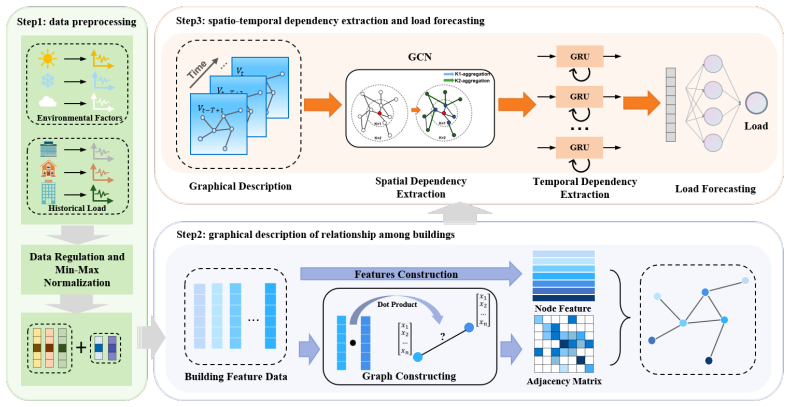
The central mechanism is the building similarity adjacency matrix $A$ with $A_{i,j} = \mathrm{ReLU}(E_i \cdot E_j)$ after top-$k$ pruning, where $E_i$ is the normalized feature vector of building $i$ (load, weather, time). This hand-constructed graph is then fed through a multi-level graph convolution; to avoid over-smoothing, an attention mechanism combines hidden states from different convolution depths, and a GRU captures temporal dependencies. The graph's role is to let each building's prediction borrow information from the buildings most similar to it.
What would settle it
Train the same Att-GCN architecture on the same data but replace the similarity graph with a randomly rewired graph and with a graph built from shuffled feature vectors; if prediction error does not worsen or does not improve over the similarity graph, the central claim that cosine-similarity spatial dependencies drive the gain is falsified.
Extended reading notes
Core claim
The paper's central claim is that a graph built from cosine similarity of building feature vectors—historical load, outdoor weather, and time indices, pruned to top-k neighbors—gives a graph neural network enough spatial structure to beat both single-building time-series models and a general-purpose graph model (MTGNN) at short-term electricity load forecasting. Reported numbers: with 20 buildings, MSE 0.0028, MAE 0.0331, R2 0.9490, SMAPE 0.0986; with 500 buildings, MSE 0.0031, MAE 0.0372, R2 0.9285, SMAPE 0.1047. The authors further claim that the trained adjacency matrix groups the 20 buildings into two clusters that coincide one-to-one with K-means clusters, and that load curves within each cluster share periodicity and trend, so the learned spatial dependencies are reasonable and interpretable.
Load-bearing premise
The load-bearing premise is that buildings whose historical load, weather, and time features are similar by cosine similarity have energy-use patterns that are predictive of each other beyond what each building's own history already predicts; if that conditional dependence is absent, the added graph edges could add noise rather than signal.
Editorial extensions
If this is right
- Multi-building forecasting can be treated as a graph task: adding edges between similar buildings improves accuracy over modeling each building alone.
- The attention-augmented graph convolution scales from 20 to 500 buildings without the accuracy loss that plain deep GCNs suffer from over-smoothing.
- The trained graph can be read as a diagnostic: clusters of buildings with similar consumption patterns emerge without separate clustering.
- The model's robustness under shuffled building order suggests it is using spatial structure rather than just node order.
- The generalization test on unseen buildings suggests a model trained on one set can forecast for new buildings without per-building retraining.
Reading between the lines
- A direct comparison against a null graph (randomly rewired edges or a fully connected graph) would isolate whether the gain comes from the cosine-similarity spatial assumption or from added model capacity; the paper does not run this control.
- The claimed match between learned graph clusters and K-means clusters may partly reflect that both use the same building features; a stronger test would shuffle features or learn the graph end-to-end.
- The robustness experiment shuffles building order, which changes the graph; rewiring edges while keeping node features fixed would more cleanly measure the value of the graph structure itself.
- The approach could extend to cooling, heating, or photovoltaic forecasting and to multi-step horizons, but those extensions are untested.
Editorial analysis
A structured set of objections, weighed in public.
Referee Report
Summary. The paper proposes BuildSTG, a spatio-temporal graph neural network for multi-building electricity load forecasting. The method has three stages: (i) graph representation, where a building similarity graph is built from load, weather, and time features using cosine similarity followed by top-k edge filtering; (ii) graph learning, where a multi-level GCN with attention and residual connections extracts spatial dependencies and a GRU extracts temporal dependencies; and (iii) interpretation, where the trained adjacency matrix is visualized and compared with K-means clusters. Experiments on two subsets of the Building Data Genome Project 2 dataset (20 and 500 buildings) report that Att-GCN outperforms MTGNN, XGBoost, SVR, FCNN, GRU, and Naive baselines on MSE, MAE, R2, and SMAPE. Additional experiments address robustness to feature shuffling and generalization to a new 20-building dataset.
Significance. If the reported results were unbiased, the paper would provide a useful, if incremental, application of standard STGNN components (GCN + GRU + attention) to multi-building load forecasting, with the useful addition of scale tests on 20 and 500 buildings and an interpretability analysis. The comparison against MTGNN, a strong graph-based baseline, is a positive feature, as is the inclusion of four metrics. However, the central quantitative claims are currently undermined by a temporal leakage issue: both the normalization scalers and the initial graph adjacency are computed over the full year, including the test portion, before the chronological split. In addition, the interpretability validation is circular because it clusters the same full-year features used to construct the graph. These issues affect the credibility of the headline accuracy gains, so the current manuscript does not yet provide reliable evidence for the claimed improvements.
major comments (4)
- [Section 4.1 and Section 3.3, Eq. (21)] The min-max normalization in Eq. (21) is computed over the whole year ('The data for the whole year has been normalized using min-max normalization'), and the initial adjacency matrix is also constructed 'based on the load data and outdoor environmental data for the whole year' (Section 3.3). The dataset is then split into training/validation/test in chronological order at 8:1:1. This means the test-period statistics and the test-period similarity structure are used to scale inputs and to define the graph before training. This is a form of label leakage, and the metrics in Tables 3 and 4 therefore cannot be interpreted as unbiased estimates of forecasting performance on unseen future data. The authors should recompute the normalization parameters and the graph adjacency using only the training portion (e.g., the first 80% of the year) and re-run all experiments and comparisons.
- [Section 4.2.5] The interpretability experiment validates the trained graph by comparing it with K-means clustering performed on 'the full-year load data and outdoor environment features of the 20 buildings' — the same features and the same full-year period used to construct the adjacency matrix in Section 3.3. The one-to-one correspondence between graph-based groups and K-means clusters is therefore a consistency check between two functions of the same input, not evidence that the model learned meaningful spatial dependencies. To support the interpretability claim, the comparison should use features or periods not involved in graph construction, or should compare against a null graph or a graph built from non-predictive features.
- [Section 4.2.2 and Section 4.2.4] The central claim that the hand-constructed graph adds predictive value is not tested against a null graph, a randomly wired graph, or a feature-shuffled control. The multi-building baselines GCN and MTGNN also use graphs, while the single-building baselines differ in architecture and input features, so the reported gains do not isolate the contribution of the graph structure itself. The robustness experiment in Section 4.2.4 shuffles the order of building features, which simultaneously changes the input features and the resulting adjacency matrix; it therefore does not separate the effect of graph structure from the effect of feature ordering. An ablation with an identical architecture and a random or feature-shuffled adjacency matrix is needed to support the spatial-learning interpretation.
- [Eqs. (15)-(18)] The text states that cosine similarity is used to build the graph, but Eq. (16) defines the adjacency as ReLU(E_i · E_j). These coincide only if the feature vectors are normalized to unit norm, which is not stated. If the vectors are not normalized, the adjacency encodes magnitude as well as direction, contradicting the cosine-similarity description. Please specify the exact construction, including whether the feature vectors are L2-normalized before computing Eq. (16), and use consistent notation throughout.
minor comments (5)
- [Table 2 / Section 3.3] The top-k neighbor count used in Eq. (17) for edge filtering is not reported, nor is the procedure for selecting it. Since this parameter directly controls graph sparsity, it should be listed in Table 2 with its tuning method.
- [Tables 3 and 4] The reported metrics are single-point averages without standard deviations or repeated-run variability. Given the small differences between some methods (e.g., Att-GCN vs. GCN), reporting means and standard deviations over multiple random seeds would help assess significance.
- [Section 4.2.4] The generalization test lacks essential details: it does not specify which dataset (20-building or 500-building) the model was trained on, how the 'new' 20 buildings were selected to avoid overlap, or whether any hyperparameters were re-tuned. These details should be added for reproducibility.
- [Section 3.4, Eq. (14)] In Eq. (14), the notation is inconsistent: the output is written as Y but the text and surrounding context refer to the predicted value \hat{Y}. Please correct the symbol.
- [Section 5] The conclusion contains a garbled list of improvement percentages ('outperforms the traditional GCN by 10.3%, 50.4%, 9.6% and 15.2%, 12.6%'), which does not match the values in Tables 3 and 4 and should be rewritten.
Circularity Check
The interpretability validation is self-referential because both the graph and the K-means comparison are computed from the same full-year features, and the reported forecast evaluations are contaminated by whole-year normalization and graph construction that include the test period.
-
self definitional
[Section 3.3 (Eqs. 15-18) and Section 4.2.5]
"Before the model training, the initialized adjacency matrix is constructed based on the load data and outdoor environmental data for the whole year ... Meanwhile, K-means clustering was conducted on the full-year load data and outdoor environment features of the 20 buildings. ... the buildings in each category correspond one-to-one. This congruency underscores the efficiency of the proposed model in identifying different types of buildings based on building features."
The interpretability claim is that the trained graph's clusters match K-means clusters and therefore prove that the model learned meaningful spatial dependencies. But the initialized adjacency matrix (Eqs. 15-18) is built from exactly the same full-year load and outdoor-environment features on which K-means is run. The one-to-one agreement is therefore largely an automatic consequence of clustering the same input vectors twice, not independent evidence that training discovered spatial structure; it validates the graph constructor against itself.
-
fitted input called prediction
[Section 3.3 and Section 4.1 (Eq. 21)]
"Before the model training, the initialized adjacency matrix is constructed based on the load data and outdoor environmental data for the whole year ... The data for the whole year has been normalized using min-max normalization ... The data is divided into training, testing, and validation sets in a time-sequential order at a ratio of 8:1:1."
Tables 3-4 present Att-GCN's test-period MSE, MAE, R2, and SMAPE as predictions, but both the min-max scalers of Eq. (21) and the adjacency matrix A are computed from the entire year, which includes the 10% test segment. The model's graph structure and input scaling are therefore informed by the very period it is asked to forecast, so the reported accuracy gains are not obtained from a purely causal forecast and are partly forced by future-period information entering the input construction.
full rationale
The accuracy comparison itself is not circular in the narrow sense: Att-GCN, GCN, MTGNN, and the single-building baselines are evaluated against the same test split, and no load-bearing claim is justified only by a self-citation. However, two construction-level problems reduce parts of the paper's argument. First, the interpretability experiment compares graph-derived clusters with K-means clusters computed from the same full-year features used to initialize the adjacency matrix, so the claimed one-to-one agreement is largely self-definitional rather than an independent confirmation of learned spatial structure. Second, the whole-year min-max normalization and whole-year graph construction leak test-period information into the model's inputs, making the reported forecasting improvements a partly in-sample evaluation of the graph and scalers rather than a clean out-of-sample prediction. These issues are specific and quotable, but they do not reduce the entire method to its inputs, hence the moderate score.
Assumptions & free parameters
free parameters (2)
- top-k neighbor count for edge filtering =
not reported
- Architecture hyperparameters (GCN channels, GCN hidden layers, GCN depth, GRU layers, GRU dim, attention dim, dropout) =
16, 4, 2, 2, 16, 32, 0.3
assumptions (4)
- domain assumption Buildings with similar intrinsic characteristics and environmental conditions exhibit similar energy consumption patterns.
- domain assumption Cosine similarity of normalized feature vectors is a valid measure of inter-building correlation.
- standard math The standard GCN, GRU, and attention equations presented in Section 2 are correct and applicable.
- domain assumption The Building Data Genome Project 2 hourly data adequately represents building operating conditions for forecasting.
Cite this review
Pith. "Pith review of BuildSTG: A Multi-building Energy Load Forecasting Method using Spatio-Temporal Graph Neural Network." pith.science (2026). https://pith.science/paper/Z5YOXUXI
@misc{pith2026250720838,
  author       = {Pith},
  title        = {Pith review of: BuildSTG: A Multi-building Energy Load Forecasting Method using Spatio-Temporal Graph Neural Network},
  year         = {2026},
  howpublished = {\url{https://pith.science/paper/Z5YOXUXI}},
  note         = {Machine review of arXiv:2507.20838}
}
read the original abstract
Due to the extensive availability of operation data, data-driven methods show strong capabilities in predicting building energy loads. Buildings with similar features often share energy patterns, reflected by spatial dependencies in their operational data, which conventional prediction methods struggle to capture. To overcome this, we propose a multi-building prediction approach using spatio-temporal graph neural networks, comprising graph representation, graph learning, and interpretation. First, a graph is built based on building characteristics and environmental factors. Next, a multi-level graph convolutional architecture with attention is developed for energy prediction. Lastly, a method interpreting the optimized graph structure is introduced. Experiments on the Building Data Genome Project 2 dataset confirm superior performance over baselines such as XGBoost, SVR, FCNN, GRU, and Naive, highlighting the method's robustness, generalization, and interpretability in capturing meaningful building similarities and spatial relationships.
Figures


Figures from the paper (6 more)


Reference graph
Works this paper leans on
-
[1]
U. N. E. Programme, Global status report for buildings and construction: Beyond foundations mainstreaming sus- tainable solutions to cut emissions from the buildings sec- tor, Website, 2024. https://www.unep.org/resources/report/ global-status-report-buildings-and-construction
work page 2024
-
[2]
Z. Li, J. Dai, H. Chen, B. Lin, An ann-based fast building energy consumption prediction method for complex architectural form at the early design stage, in: Building Simulation, volume 12, Springer, 2019, pp. 665–681. 27
work page 2019
-
[3]
M. Ilbeigi, M. Ghomeishi, A. Dehghanbanadaki, Prediction and op- timization of energy consumption in an office building using artificial neural network and a genetic algorithm, Sustainable Cities and Society 61 (2020) 102325
work page 2020
- [4]
-
[5]
A. A. A. Gassar, S. H. Cha, Energy prediction techniques for large-scale buildings towards a sustainable built environment: A review, Energy and Buildings 224 (2020) 110238
work page 2020
-
[6]
Q. Tan, C. Cao, G. Xue, W. Xie, Short-term heating load forecasting model based on svmd and improved informer, Energy 312 (2024) 133535
work page 2024
-
[7]
Z. Gao, S. Yang, J. Yu, A. Zhao, Hybrid forecasting model of building cooling load based on combined neural network, Energy 297 (2024) 131317
work page 2024
-
[8]
C. Fan, F. Xiao, Y. Zhao, A short-term building cooling load prediction method using deep learning algorithms, Applied energy 195 (2017) 222– 233
work page 2017
Show all 46 references
-
[9]
J. Wang, X. Chen, F. Zhang, F. Chen, Y. Xin, Building load forecast- ing using deep neural network with efficient feature fusion, Journal of Modern Power Systems and Clean Energy 9 (2021) 160–169
2021
-
[10]
H. Bian, Q. Wang, G. Xu, X. Zhao, Research on short-term load fore- casting based on accumulated temperature effect and improved temporal convolutional network, Energy Reports 8 (2022) 1482–1491
2022
-
[11]
S. Jung, J. Moon, S. Park, E. Hwang, An attention-based multilayer gru model for multistep-ahead short-term load forecasting, Sensors 21 (2021) 1639
2021
-
[12]
Bashir, C
T. Bashir, C. Haoyong, M. F. Tahir, Z. Liqiang, Short term electricity load forecasting using hybrid prophet-lstm model optimized by bpnn, Energy reports 8 (2022) 1678–1686. 28
2022
-
[13]
Berardi, A cross-country comparison of the building energy con- sumptions and their trends, Resources, Conservation and Recycling 123 (2017) 230–241
U. Berardi, A cross-country comparison of the building energy con- sumptions and their trends, Resources, Conservation and Recycling 123 (2017) 230–241
2017
-
[14]
Gupta, S
G. Gupta, S. Mathur, J. Mathur, B. K. Nayak, Comparison of energy- efficiency benchmarking methodologies for residential buildings, Energy and Buildings 285 (2023) 112920
2023
-
[15]
Saeedi, M
M. Saeedi, M. Moradi, M. Hosseini, A. Emamifar, N. Ghadimi, Ro- bust optimization based optimal chiller loading under cooling demand uncertainty, Applied Thermal Engineering 148 (2019) 1081–1091
2019
-
[16]
Zhang, Y
C. Zhang, Y. Zhao, C. Fan, T. Li, X. Zhang, J. Li, A generic pre- diction interval estimation method for quantifying the uncertainties in ultra-short-term building cooling load prediction, Applied Thermal En- gineering 173 (2020) 115261
2020
-
[17]
Z. Wu, S. Pan, F. Chen, G. Long, C. Zhang, S. Y. Philip, A compre- hensive survey on graph neural networks, IEEE transactions on neural networks and learning systems 32 (2020) 4–24
2020
-
[18]
Arastehfar, M
S. Arastehfar, M. Matinkia, M. R. Jabbarpour, Short-term residential load forecasting using graph convolutional recurrent neural networks, Engineering Applications of Artificial Intelligence 116 (2022) 105358
2022
-
[19]
W. Lin, D. Wu, B. Boulet, Spatial-temporal residential short-term load forecasting via graph neural networks, IEEE Transactions on Smart Grid 12 (2021) 5373–5384
2021
-
[20]
Z. Wu, S. Pan, G. Long, J. Jiang, C. Zhang, Graph wavenet for deep spatial-temporal graph modeling, Proceedings of the Twenty-Eighth In- ternational Joint Conference on Artificial Intelligence (IJCAI-19) (2019)
2019
-
[21]
Y. Wang, L. Rui, J. Ma, et al., A short-term residential load fore- casting scheme based on the multiple correlation-temporal graph neural networks, Applied Soft Computing 146 (2023) 110629
2023
-
[22]
B. Yu, H. Yin, Z. Zhu, Spatio-temporal graph convolutional networks: A deep learning framework for traffic forecasting, Proceedings of the Twenty-Seventh International Joint Conference on Artificial Intelligence (IJCAI-18) (2018). 29
2018
-
[23]
G. Jin, Y. Liang, Y. Fang, Z. Shao, J. Huang, J. Zhang, Y. Zheng, Spatio-temporal graph neural networks for predictive learning in urban computing: A survey, IEEE Transactions on Knowledge and Data En- gineering 36 (2023) 5388–5408
2023
-
[24]
T. N. Kipf, M. Welling, Semi-supervised classification with graph con- volutional networks, Proceedings of the 34th International Conference on Machine Learning (ICML’17 (2017)
2017
-
[25]
Gilmer, S
J. Gilmer, S. S. Schoenholz, P. F. Riley, O. Vinyals, G. E. Dahl, Neural message passing for quantum chemistry, in: International conference on machine learning, PMLR, 2017, pp. 1263–1272
2017
-
[26]
T. Pham, T. Tran, H. Dam, S. Venkatesh, Graph classification via deep learning with virtual nodes, arXiv preprint arXiv:1708.04357 (2017)
2017 arXiv
-
[27]
Z. Ying, J. You, C. Morris, X. Ren, W. Hamilton, J. Leskovec, Hierarchi- cal graph representation learning with differentiable pooling, Advances in neural information processing systems 31 (2018)
2018
-
[28]
Y. Ma, S. Wang, C. C. Aggarwal, J. Tang, Graph convolutional net- works with eigenpooling, in: Proceedings of the 25th ACM SIGKDD international conference on knowledge discovery & data mining, 2019, pp. 723–731
2019
-
[29]
J. L. Elman, Finding structure in time, Cognitive science 14 (1990) 179–211
1990
-
[30]
Hochreiter, J
S. Hochreiter, J. Schmidhuber, Long short-term memory, Neural com- putation 9 (1997) 1735–1780
1997
-
[31]
K. Cho, B. Van Merri¨ enboer, C. Gulcehre, D. Bahdanau, F. Bougares, H. Schwenk, Y. Bengio, Learning phrase representations using rnn encoder-decoder for statistical machine translation, Proceedings of the 2014 Conference on Empirical Methods in Natural Language Processing (EM...
2014
-
[32]
Vaswani, N
A. Vaswani, N. Shazeer, N. Parmar, J. Uszkoreit, L. Jones, A. N. Gomez, L. Kaiser, I. Polosukhin, Attention is all you need, Advances in neural information processing systems 30 (2017). 30
2017
-
[33]
Gross, F
G. Gross, F. D. Galiana, Short-term load forecasting, Proceedings of the IEEE 75 (2005) 1558–1573
2005
-
[34]
P.-N. Tan, M. Steinbach, V. Kumar, Introduction to data mining, Pear- son Education India, 2016
2016
-
[35]
Q. Li, Z. Han, X.-M. Wu, Deeper insights into graph convolutional networks for semi-supervised learning, in: Proceedings of the AAAI conference on artificial intelligence, volume 32, 2018
2018
-
[36]
K. He, X. Zhang, S. Ren, J. Sun, Deep residual learning for image recognition, in: Proceedings of the IEEE conference on computer vision and pattern recognition, 2016, pp. 770–778
2016
-
[37]
Miller, A
C. Miller, A. Kathirgamanathan, B. Picchetti, P. Arjunan, J. Y. Park, Z. Nagy, P. Raftery, B. W. Hobson, Z. Shi, F. Meggers, The building data genome project 2, energy meter data from the ashrae great energy predictor iii competition, Scientific data 7 (2020) 368
2020
-
[38]
T. Chen, C. Guestrin, Xgboost: A scalable tree boosting system, in: Proceedings of the 22nd acm sigkdd international conference on knowl- edge discovery and data mining, 2016, pp. 785–794
2016
-
[39]
Platt, Sequential minimal optimization: A fast algorithm for training support vector machines (1998)
J. Platt, Sequential minimal optimization: A fast algorithm for training support vector machines (1998)
1998
-
[40]
Drucker, C
H. Drucker, C. J. Burges, L. Kaufman, A. Smola, V. Vapnik, Support vector regression machines, Advances in neural information processing systems 9 (1996)
1996
-
[41]
Z. Wu, S. Pan, G. Long, J. Jiang, X. Chang, C. Zhang, Connecting the dots: Multivariate time series forecasting with graph neural networks,
-
[42]
https://pytorch.org/
Pytorch, Website, 2025. https://pytorch.org/
2025
-
[43]
D. P. Kingma, J. Ba, Adam: A method for stochastic optimization, arXiv preprint arXiv:1412.6980 (2014)
2014 arXiv
-
[44]
P. J. Rousseeuw, Silhouettes: a graphical aid to the interpretation and validation of cluster analysis, Journal of computational and applied mathematics 20 (1987) 53–65. 31
1987
-
[45]
Van der Maaten, G
L. Van der Maaten, G. Hinton, Visualizing data using t-sne., Journal of machine learning research 9 (2008). Appendix A. (a) (b) Figure A1: The structure of the related methods: (a) A GRU cell. (b) The attention mechanism. 32
2008
- [2020]
Reviewed August 6, 2026 · model on record in the stance chip above.
Discussion (0). Sign in to comment.