A prism hierarchy of learning regimes in large linear autoencoders

Dmitry Yarotsky; Eugene Golikov; Yaroslav Gusev

arxiv: 2606.05335 · v1 · pith:ZDHUWMC2new · submitted 2026-06-03 · 💻 cs.LG · stat.ML

A prism hierarchy of learning regimes in large linear autoencoders

Eugene Golikov , Yaroslav Gusev , Dmitry Yarotsky This is my paper

Pith reviewed 2026-06-28 07:23 UTC · model grok-4.3

classification 💻 cs.LG stat.ML

keywords linear autoencodersgradient flowextreme regimesloss expansionprism hierarchymean-field limitlarge data regimeweight-tied models

0 comments

The pith

Extreme regimes of large linear autoencoders map to faces of a triangular prism.

A machine-rendered reading of the paper's core claim, the machinery that carries it, and where it could break.

The paper seeks a systematic classification of all qualitatively distinct extreme learning regimes for large weight-tied linear autoencoders, which depend on input dimension, latent dimension, initialization magnitude, and training set size. At the level of a formal hierarchy of loss expansions, these regimes correspond to the faces of a triangular prism, yielding five basic extreme cases on the two-dimensional faces. Explicit expressions for the limiting evolution of both training and population losses under gradient flow are derived for four of the regimes. These expressions match numerical experiments closely. The approach replaces isolated limiting-case analyses with a unified geometric organization of the parameter space.

Core claim

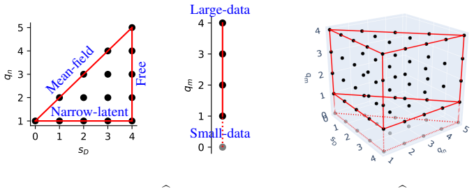
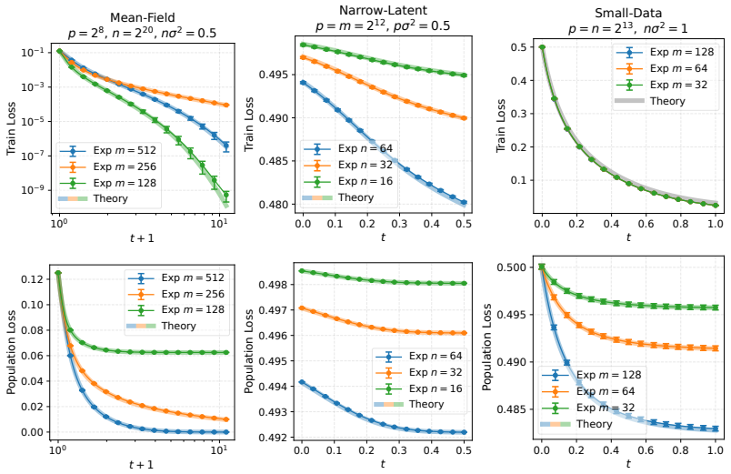
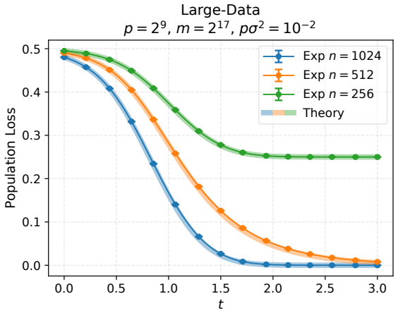
At the level of the formal loss-expansion hierarchy, the extreme regimes of large weight-tied linear autoencoders are naturally associated with faces of a triangular prism. In particular, there are five basic extreme regimes associated with the 2-faces: large-data, small-data, mean-field, narrow-latent, and free. For the first four regimes, explicit expressions are derived for both train and population limiting loss evolutions under gradient flow.

What carries the argument

The triangular prism hierarchy, in which each face corresponds to a distinct scaling regime of the input dimension, latent dimension, initialization, and dataset size that produces a separate limiting form of the loss expansion.

If this is right

Both training and population losses admit explicit closed-form limiting expressions in the large-data, small-data, mean-field, and narrow-latent regimes.
The derived expressions agree closely with direct simulations of gradient flow on large weight-tied linear autoencoders.
The five extreme regimes cover the qualitatively different behaviors at the extremes of the parameter space defined by input size, latent size, initialization, and data size.
The prism structure provides a geometric organization that unifies previously separate limiting analyses.

Where Pith is reading between the lines

These are editorial extensions of the paper, not claims the author makes directly.

The prism geometry may suggest similar hierarchical structures in other models where loss expansions can be ordered by scaling parameters.
Targeting a specific face of the prism could guide selection of initialization or architecture to reach a regime with reliable theoretical predictions.
The free regime without an explicit derivation may require separate analysis techniques to obtain closed-form limits.

Load-bearing premise

The formal loss-expansion hierarchy is assumed to be sufficient to identify all qualitatively distinct extreme regimes without missing important dynamical effects arising from the nonlinear dependence on the weights.

What would settle it

A numerical experiment in which the observed train or population loss trajectory in one of the four derived regimes deviates substantially from the explicit limiting expression would falsify the claim.

Figures

Figures reproduced from arXiv: 2606.05335 by Dmitry Yarotsky, Eugene Golikov, Yaroslav Gusev.

**Figure 2.** Figure 2: The triangular prisms Ps, Pbs describing the Pareto monomials in Ys, Ybs (see Theorem 3.2) for s = 3. The solid lines show the common parts of Ps, Pbs (qm ≥ 1), while the dotted lines show the bottom qm = 0 only present in Pbs. The five regimes correspond to the five 2-faces of the prism. 2. At s = 0, the population Pareto set P0 = Pb0. At s ≥ 1, Ps is obtained from Pbs by removing the points with qm = 0. … view at source ↗

**Figure 3.** Figure 3: Empirical validation of the limiting predictions (Sec. 4) across different regimes. Markers [PITH_FULL_IMAGE:figures/full_fig_p006_3.png] view at source ↗

**Figure 4.** Figure 4: Empirical validation of the limiting predictions for large-data regime. [PITH_FULL_IMAGE:figures/full_fig_p032_4.png] view at source ↗

read the original abstract

Theoretical studies of machine learning models commonly consider different limiting regimes in which the learning dynamics of gradient descent becomes theoretically tractable. It is, however, desirable to have a systematically obtained picture of all qualitatively different extreme learning regimes for a particular type of models. In this paper we propose such a picture for large weight-tied linear autoencoders characterized by input and latent dimensions, initialization magnitude, and training set size. This model is nonlinear in the weights and its gradient flow does not have a general theoretical solution. We show that at the level of the formal loss-expansion hierarchy, its extreme regimes are naturally associated with faces of a triangular prism. In particular, there are five basic extreme regimes associated with the 2-faces of the prism: (1) large-data, (2) small-data, (3) mean-field, (4) narrow-latent, and (5) free. For regimes (1,2,3,4), we derive explicit expressions for both train and population limiting loss evolutions under gradient flow, obtaining very good agreement with experimental results.

Editorial analysis

A structured set of objections, weighed in public.

Desk editor's note, referee report, simulated authors' rebuttal, and a circularity audit. Tearing a paper down is the easy half of reading it; the pith above is the substance, this is the friction.

Desk Editor's Note private letter to a colleague

The prism organizes five regimes for weight-tied linear autoencoders and supplies explicit loss formulas for four of them that match experiments.

read the letter

The main takeaway is that the paper maps the extreme regimes of large weight-tied linear autoencoders onto the faces of a triangular prism and derives explicit train and population loss trajectories under gradient flow for four of the five cases.

The contribution is the systematic classification itself. The model is nonlinear in its weights, so gradient flow has no general solution. They apply a loss-expansion hierarchy to identify the distinct limits and tie them to the 2-faces: large-data, small-data, mean-field, narrow-latent, and free. Closed-form expressions appear for the first four, and the abstract states these match numerical runs well. That match is the concrete evidence offered.

The soft spot is the reliance on the expansion hierarchy being complete. Because the dynamics are nonlinear, higher-order terms or mixed scalings could in principle produce behavior not captured by the prism faces. The free regime receives no explicit derivation, which leaves one corner less developed. The abstract does not include the full steps or error bounds, so a referee would need to check whether the truncation is justified beyond the tested corners.

This is for people working on scaling laws and mean-field analyses in linear or linearized models. A reader who wants a single geometric picture that links several standard limits will find it useful. The work deserves peer review because the claim is specific, the experimental support is reported as strong, and the prism framing is a clean organizing device even if the hierarchy assumption needs scrutiny.

Referee Report

2 major / 1 minor

Summary. The paper claims that extreme learning regimes for large weight-tied linear autoencoders (parameterized by input/latent dimensions, initialization magnitude, and training set size) are systematically organized by a formal loss-expansion hierarchy into faces of a triangular prism. Five basic extreme regimes are associated with the 2-faces: (1) large-data, (2) small-data, (3) mean-field, (4) narrow-latent, and (5) free. Explicit expressions for both train and population limiting loss evolutions under gradient flow are derived for regimes (1-4), with very good agreement to experiments.

Significance. If the hierarchy is complete and the limiting expressions hold, the work offers a systematic classification of qualitatively distinct regimes for a nonlinear model whose gradient flow lacks a general closed form. The explicit derivations for four regimes and their experimental matches provide concrete, falsifiable predictions for loss trajectories across scaling limits, which is a strength for theoretical ML analysis.

major comments (2)

Abstract: the central claim that explicit expressions for limiting train/population losses were derived for regimes (1,2,3,4) and match experiments well cannot be verified without the loss-expansion steps, truncation error analysis, or details on how the hierarchy classifies the nonlinear dynamics; this is load-bearing for the explicit expressions.
Abstract: the assertion that the five 2-face regimes exhaust the qualitatively distinct extreme limits assumes the formal loss-expansion hierarchy is complete, but the manuscript provides no argument or test ruling out additional dynamical effects from higher-order interactions or mixed scalings not aligned with prism axes.

minor comments (1)

The abstract refers to 'very good agreement with experimental results' without specifying quantitative metrics, error bounds, or which figures/tables demonstrate the match.

Simulated Author's Rebuttal

2 responses · 0 unresolved

We thank the referee for their careful reading and for highlighting points that strengthen the presentation of our results. We respond to each major comment below.

read point-by-point responses

Referee: Abstract: the central claim that explicit expressions for limiting train/population losses were derived for regimes (1,2,3,4) and match experiments well cannot be verified without the loss-expansion steps, truncation error analysis, or details on how the hierarchy classifies the nonlinear dynamics; this is load-bearing for the explicit expressions.

Authors: The loss-expansion steps, truncation error bounds, and the mapping from prism faces to dynamical regimes are derived in Sections 3–6 and Appendices A–C. These sections show how the nonlinear gradient-flow equations reduce to closed-form ODEs under each scaling. We will revise the abstract to include a parenthetical pointer to these sections so that the central claim can be traced directly to the supporting derivations. revision: partial
Referee: Abstract: the assertion that the five 2-face regimes exhaust the qualitatively distinct extreme limits assumes the formal loss-expansion hierarchy is complete, but the manuscript provides no argument or test ruling out additional dynamical effects from higher-order interactions or mixed scalings not aligned with prism axes.

Authors: Within the formal loss-expansion framework the five 2-faces correspond to the leading-order balances obtained by taking each of the four parameters to its extreme while holding the others fixed; any mixed scaling either collapses to one of these faces or produces only sub-dominant corrections that do not alter the qualitative loss trajectory. We will add a short subsection (new Section 2.4) that makes this reduction argument explicit and notes that higher-order interaction terms remain negligible under the same scaling assumptions used for the four explicit derivations. revision: partial

Circularity Check

0 steps flagged

Derivations from loss-expansion hierarchy are self-contained

full rationale

The paper applies a formal loss-expansion hierarchy to the weight-tied linear autoencoder to classify extreme regimes as prism faces and derives explicit train/population loss trajectories under gradient flow for four of the five 2-face regimes. These derivations are presented as direct consequences of the hierarchy truncation at the relevant scaling limits, with external experimental validation. No quoted step reduces a claimed prediction to a fitted parameter by construction, renames a known result, or relies on a load-bearing self-citation whose content is itself unverified. The hierarchy is treated as an independent organizing tool rather than being defined circularly in terms of the target regimes.

Axiom & Free-Parameter Ledger

0 free parameters · 1 axioms · 1 invented entities

The central claim rests on the loss-expansion hierarchy being able to capture regime distinctions and on the four model parameters being the relevant axes; no free parameters or new physical entities are introduced in the abstract.

axioms (1)

domain assumption Gradient flow on the nonlinear loss of the weight-tied linear autoencoder can be analyzed via a formal loss-expansion hierarchy that identifies distinct extreme regimes.
Invoked to associate regimes with prism faces and derive limiting dynamics.

invented entities (1)

triangular prism hierarchy of regimes no independent evidence
purpose: To organize the five extreme learning regimes geometrically
Conceptual structure introduced by the paper to map parameter limits to dynamical behaviors.

pith-pipeline@v0.9.1-grok · 5722 in / 1296 out tokens · 44851 ms · 2026-06-28T07:23:20.480340+00:00 · methodology

discussion (0)

Reference graph

Works this paper leans on

13 extracted references

[1]

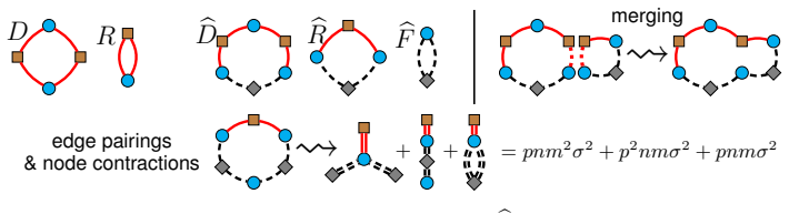
The vertices correspond to the summation indices and can be one of the three types: p (input dimension),n(latent dimension) orm(dataset size)
[2]

U-edges connect n-nodes with p-nodes, whileX-edges connectp-nodes withm-nodes

The edges connecting two vertices correspond to respective entries of the matrices U,X and accordingly can be of two types ( U or X). U-edges connect n-nodes with p-nodes, whileX-edges connectp-nodes withm-nodes
[3]

Note that: 14

The value associated with the diagram is obtained by multiplying the entries of U,X over the edges and summing resulting products over all configurations of node indices. Note that: 14
[4]

Thanks to the trace-product structure of D, R,bD,bR,bF , the associated five diagrams are ring diagrams(see Fig. 1). However, in general diagrams defined by above rules may be more general, e.g. the diagrams obtained by contractions of the ring diagrams (see below) are not ring diagrams
[5]

The number of X-edges is twice the number of m-nodes, while the number of U-edges is twice the number ofn-nodes

In the ring diagrams such as D, R,bD,bR,bF , the n, m-nodes alternate with p-nodes. The number of X-edges is twice the number of m-nodes, while the number of U-edges is twice the number ofn-nodes. Diagram merging.Computation of scalar products (37) can be described in terms ofdiagram merging. Let G1, G2 be two functions of the weights represented by diagr...
[6]

Consider all pairs of aU-edgeg 1 inG 1 and aU-edgeg 2 inG 2
[7]

For each such pair, merge the diagrams G1 and G2 by identifying the n-nodes of g1, g2, identifying thep-nodes ofg 1, g2, and removing the edgesg 1, g2 (see Fig. 1)
[8]

Note that:

Add the resulting diagrams. Note that:
[9]

Merger of two diagrams produces a linear combination of diagrams (corresponding to different pairs of edges)
[10]

The diagrams are merged only over U-edges and not X-edges (since only the U-edges contain the trainable model weights)
[11]

Let q(r) p , q(r) n , q(r) m , q(r) σ denote, respectively, the numbers of p-, n-, m-nodes and edges in Gr, r= 0,1

Merger of two ring diagrams G1, G2 produces again ring diagrams. Let q(r) p , q(r) n , q(r) m , q(r) σ denote, respectively, the numbers of p-, n-, m-nodes and edges in Gr, r= 0,1 . Then in the merged diagrams qp =q (1) p +q (2) p −1,(42) qn =q (1) n +q (2) n −1,(43) qm =q (1) m +q (2) m ,(44) qσ =q (1) σ +q (2) σ −2.(45) We denote the merge operation by⋆...
[12]

Consider all pairings of the edges ofG between matching edges (i.e., U-edges with U-edges andX-edges withX-edges)
[13]

spectral overfitting

For each pairing: (a) For each pair of edges,contract(i,e., identify) their respective p-, n- and/or m-nodes. The resulting contracted nodes correspond to the degrees of freedom left after imposing all the identity constraints. (b) The resulting contracted diagram contributes to E[G] the term pqp nqn mqm σqσ , where qp, qn, qm are the numbers of respectiv...

2026

[1] [1]

The vertices correspond to the summation indices and can be one of the three types: p (input dimension),n(latent dimension) orm(dataset size)

[2] [2]

U-edges connect n-nodes with p-nodes, whileX-edges connectp-nodes withm-nodes

The edges connecting two vertices correspond to respective entries of the matrices U,X and accordingly can be of two types ( U or X). U-edges connect n-nodes with p-nodes, whileX-edges connectp-nodes withm-nodes

[3] [3]

Note that: 14

The value associated with the diagram is obtained by multiplying the entries of U,X over the edges and summing resulting products over all configurations of node indices. Note that: 14

[4] [4]

Thanks to the trace-product structure of D, R,bD,bR,bF , the associated five diagrams are ring diagrams(see Fig. 1). However, in general diagrams defined by above rules may be more general, e.g. the diagrams obtained by contractions of the ring diagrams (see below) are not ring diagrams

[5] [5]

The number of X-edges is twice the number of m-nodes, while the number of U-edges is twice the number ofn-nodes

In the ring diagrams such as D, R,bD,bR,bF , the n, m-nodes alternate with p-nodes. The number of X-edges is twice the number of m-nodes, while the number of U-edges is twice the number ofn-nodes. Diagram merging.Computation of scalar products (37) can be described in terms ofdiagram merging. Let G1, G2 be two functions of the weights represented by diagr...

[6] [6]

Consider all pairs of aU-edgeg 1 inG 1 and aU-edgeg 2 inG 2

[7] [7]

For each such pair, merge the diagrams G1 and G2 by identifying the n-nodes of g1, g2, identifying thep-nodes ofg 1, g2, and removing the edgesg 1, g2 (see Fig. 1)

[8] [8]

Note that:

Add the resulting diagrams. Note that:

[9] [9]

Merger of two diagrams produces a linear combination of diagrams (corresponding to different pairs of edges)

[10] [10]

The diagrams are merged only over U-edges and not X-edges (since only the U-edges contain the trainable model weights)

[11] [11]

Let q(r) p , q(r) n , q(r) m , q(r) σ denote, respectively, the numbers of p-, n-, m-nodes and edges in Gr, r= 0,1

Merger of two ring diagrams G1, G2 produces again ring diagrams. Let q(r) p , q(r) n , q(r) m , q(r) σ denote, respectively, the numbers of p-, n-, m-nodes and edges in Gr, r= 0,1 . Then in the merged diagrams qp =q (1) p +q (2) p −1,(42) qn =q (1) n +q (2) n −1,(43) qm =q (1) m +q (2) m ,(44) qσ =q (1) σ +q (2) σ −2.(45) We denote the merge operation by⋆...

[12] [12]

Consider all pairings of the edges ofG between matching edges (i.e., U-edges with U-edges andX-edges withX-edges)

[13] [13]

spectral overfitting

For each pairing: (a) For each pair of edges,contract(i,e., identify) their respective p-, n- and/or m-nodes. The resulting contracted nodes correspond to the degrees of freedom left after imposing all the identity constraints. (b) The resulting contracted diagram contributes to E[G] the term pqp nqn mqm σqσ , where qp, qn, qm are the numbers of respectiv...

2026