REVIEW 2 major objections 4 minor 101 references
Geometry of quantum states and chaos-integrability transition
T0 review · 2 major / 4 minor · reviewed 2026-08-06 · deepseek-v4-flash
Pith's one-line read A finite geodesic distance links integrability and chaos in random-matrix models.
desk verdict Solid analytical additions to quantum state geometry, but the central finite-geodesic-distance claim is undercut by inconsistent constants in the key figures and an overbroad abstract. read the letter →
The pith
A machine-rendered reading of the paper's core claim, the machinery that carries it, and where it could break.
The reading
What carries the argument
The central object is the ensemble-averaged quantum metric tensor (QMT), the real part of the quantum geometric tensor pulled back to the parameter space of the Hamiltonian. For the integrability-breaking Hamiltonian it is evaluated in a 2x2 representation, giving the line element ds² = g_rr dr² + g_φφ dφ²; the key simplification is the coordinate change r=√2 cot θ, which maps the integrable limit to θ=π/2 and the chaotic limit to θ=0 and makes the geodesic equation tractable. The second main mechanism is the identity expressing the fidelity susceptibility as an integral of the connected two-point correlation function, 1/(E_j−E_n)² = ∫ dω/ω² ∫ dt/(2π) $e^{{−i(E_j−E_n−ω)t}}$, which ties the metric to the spectral form factor.
What would settle it
Numerically integrate the first-order geodesic equation using the large-N quantum metric tensor scalings of the generalized Rosenzweig-Porter model (for instance the 1/r behaviour in the localized phase) and check whether r(λ) diverges at a finite affine parameter; if the geodesic distance to r→∞ diverges for any initial condition, the finite-distance claim fails.
Extended reading notes
Core claim
The central claim is that for the ensemble-averaged quantum metric tensor of a 2x2 generalized Rosenzweig-Porter Hamiltonian, any parameter point arbitrarily far from the integrable limit can be reached by a finite geodesic distance. The argument proceeds by transforming to coordinates r=√2 cot θ, reducing the geodesic equation to a first-order form, and solving it approximately to obtain r(λ)=−√2 cot[√(A1/A2) tan(√(A1A2)λ − arctan(√(A2/A1)θ0))], which diverges at a finite affine parameter. The paper further shows that the fidelity susceptibility obtained from GUE correlation functions reproduces the quantum metric component, with the spectral form factor supplying the N-dependent part, and that the fidelity susceptibility of tridiagonal Gaussian beta-ensembles diverges as 1/r when approaching the integrable point for any β>1.
Load-bearing premise
The result's load-bearing premise is that the 2x2 calculation captures the geodesic behaviour of the true large-N model, since analytic quantum metric tensor components for arbitrary N are not known and only numerical scalings exist.
Editorial extensions
If this is right
- The geodesic distance of the averaged QMT can serve as a computable complexity measure for reaching chaos from integrability, at least in the two-parameter setup.
- The fidelity susceptibility is expressible directly in terms of the spectral form factor, so spectral statistics determines the state-space geometry for GUE-type Hamiltonians.
- For Gaussian beta-ensembles with any β>1, the fidelity susceptibility diverges as 1/r near integrability, showing a universal geometric signature of the transition.
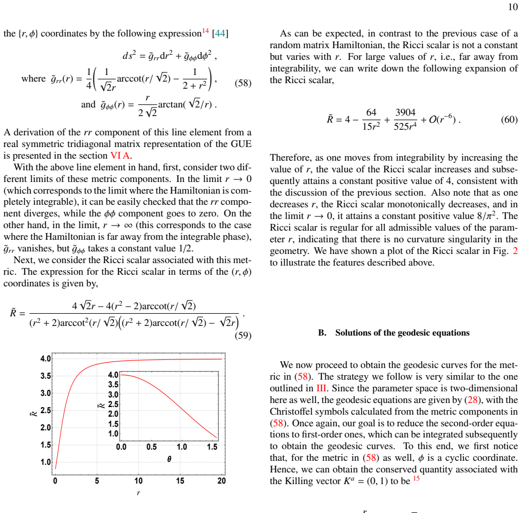
- The Ricci scalar of the averaged QMT changes from a constant in the chaotic GUE phase to a parameter-dependent function when unitary symmetry is broken, tracking the symmetry-breaking strength.
- The same geometric framework can be extended to non-Hermitian Hamiltonians, where the bi-orthogonal inner product is expected to produce a richer tensor structure.
Reading between the lines
- If the finite-geodesic-distance result survives at large N, it would imply that the parameter manifold of these random-matrix ensembles has no barrier separating integrable and chaotic phases, unlike Lipkin-Meshkov-Glick-type models where the separatrix is at infinite distance.
- The 1/r divergence of the fidelity susceptibility near integrability may serve as a diagnostic that distinguishes integrability-breaking transitions from ordinary quantum phase transitions, which typically show power-law or logarithmic singularities.
- A direct test would be to numerically integrate the geodesic equation using the large-N QMT scalings reported for the generalized Rosenzweig-Porter model and check whether r(λ) diverges at finite λ in the ergodic phase.
- The relation between the fidelity susceptibility and the spectral form factor suggests that eigenstate geometry could be probed experimentally through spectral form factor measurements in systems with tunable integrability breaking.
Editorial analysis
A structured set of objections, weighed in public.
Referee Report
Summary. The paper develops a geometric characterization of chaos-to-integrability transitions for random-matrix Hamiltonians. It computes the ensemble-averaged quantum metric tensor (QMT) for a GUE family with two parameters, shows that the metric is sphere-like, solves the geodesic equations, and derives the fidelity susceptibility (FS) from a two-point correlation function connected to the spectral form factor. It then studies a 2×2 Rosenzweig-Porter-like integrability-breaking Hamiltonian, derives its averaged QMT, and uses an approximate small-angle geodesic solution to argue that any point arbitrarily far from the integrable phase is reachable within finite geodesic distance. The paper also computes the FS for the 2×2 tridiagonal Gaussian β-ensemble for generic Dyson index β, for a rotationally invariant ensemble with an effective Dyson index, and analyzes ensemble-averaged level curvatures.
Significance. The cleanest parts of the paper are the GUE sector: the correlation-function computation, the connection between the spectral form factor and the fidelity susceptibility, and the recovery of Eq. (50) via Dyson's virial theorem are sound and pedagogically useful. The closed-form β-ensemble fidelity susceptibility in Eq. (75) is also a useful addition. The central novelty—finite geodesic distance to the chaotic phase in the broken-invariance model—is interesting, but as it stands it is established only for the N=2 averaged metric and it relies on an approximate geodesic solution whose stated parameter values lead to imaginary constants and negative kinetic terms. The paper contains no fitted parameters except an illustrative 1/r² fit in Section VII, which is not load-bearing. These issues are fixable, but they require substantive revision.
major comments (2)
- [Abstract; §V; Conclusions item 1] The finite-geodesic-distance claim is presented in the abstract and in Conclusions item 1 without the N=2 qualifier that the derivation actually requires. The calculation in §V.B is performed entirely for the 2×2 averaged QMT of Eq. (58), and the paragraph after Fig. 6 explicitly states that analytic QMT components for arbitrary N are not known, citing Ref. [44] for different scaling regimes, including a 1/r scaling in the localized phase. For a metric with g_rr ~ c/r on an unbounded interval, the radial geodesic distance ∫√(c/r) dr diverges, so finite geodesic distance is not an automatic consequence of those scalings. The advertised generality is therefore unsupported unless the authors supply a large-N argument or explicitly restrict the claim to the N=2 model.
- [§V.B, Eqs. (65)-(68), Figs. 4-6] The numerical and approximate solutions used to establish finite geodesic distance are not real for the stated parameters. With K̃ = L̃ = 0.1, the bracket in Eq. (65) at θ₀ = π/3 equals K̃² − 2L̃²/(θ₀ tan θ₀) ≈ 0.01 − 0.0110 < 0, and at θ₀ = π/4 it is ≈ 0.01 − 0.0255 < 0, so no real initial θ̇ exists for the plotted 'initially decaying' geodesics. Moreover, A₁ = √(6(K̃² − 2L̃²)) in Eq. (66) is imaginary for K̃ = L̃, and the expression for A₂ has a negative radicand. For small θ the exact right-hand side of Eq. (65) contains a negative term of order −12L̃²/θ² that is dropped in the O(θ²) expansion, so Eq. (66) cannot be a valid small-θ expansion for L̃ ≠ 0. Since Eqs. (67)-(68) are the analytic basis for the finite-distance claim, this inconsistency must be corrected before the central claim can be accepted.
minor comments (4)
- [§IV, text after Eq. (55)] The phrase 'in tern' should read 'in turn'.
- [§VI, first paragraph] The text contains the duplicated phrase 'are are independent Gaussian random variables'; one copy should be removed.
- [§V.B, Eq. (67)] The solution θ(λ) from Eq. (67) becomes negative after crossing θ = 0, while the coordinate range is 0 ≤ θ ≤ π/2; the authors should state explicitly that the solution is used only up to the first passage through θ = 0.
- [Figs. 3-6] The numerical integration scheme and error tolerances are not specified; a brief description would improve reproducibility.
Circularity Check
No circularity: the central derivations are self-contained; the N=2 generalization gap and an invalid parameter choice are correctness concerns, not circular reasoning.
full rationale
The paper's derivation chain is not circular. The GUE fidelity susceptibility in Sec. IV is recovered from the two-point correlation function using the spectral representation (13) derived from definitions, Dyson's external virial theorem (B4), and the known GUE resolvent (56); these are independent, parameter-free inputs that do not presuppose the target metric. The finite-geodesic-distance result for the integrability-breaking Hamiltonian is derived from the ensemble-averaged 2x2 QMT in eq. (58), which is imported from the external Ref. [44] and independently re-derived for beta=2 in Sec. VI A from the tridiagonal representation. The geodesic equation (65) and its approximate solution (67)-(68) are solved within the paper; no fitted parameter forces the divergence of r(lambda). The only self-citations, Refs. [65] and [88], are comparisons or side remarks and are not load-bearing. The paper explicitly flags the N=2 limitation in Sec. V ('analytic expressions for the QMT components for an arbitrary value of N are not known'), so the abstract-level generalization is a scope concern, not circularity. Finally, the plotted values K=0.1, L=0.1 in Figs. 4-6 make the bracket in eq. (65) negative and A1 imaginary, which is a technical/correctness issue, not a circular step.
Assumptions & free parameters
free parameters (1)
- c in \tilde{g}_{rr}(r) ≈ c/r^2 (Section VII fit) =
0.1
assumptions (6)
- standard math Dyson's virial theorem (eq. B4) for Gaussian random matrix ensembles.
- standard math Joint eigenvalue distribution (eq. 6) and Dumitriu-Edelman tridiagonal representation (eq. 69) of Gaussian beta-ensembles.
- standard math The 2x2 ensemble-averaged QMT components in eq. (58) for the integrability-breaking Hamiltonian.
- domain assumption The ensemble-averaged QMT \bar{g}_{ab} defines a Riemannian metric on the parameter manifold whose geodesics carry geometric/complexity meaning.
- ad hoc to paper The 2x2 model is representative of the N-dimensional Rosenzweig-Porter model for the geodesic-finiteness claim.
- domain assumption The total Hamiltonian H(r) has no degenerate spectrum.
Cite this review
Pith. "Pith review of Geometry of quantum states and chaos-integrability transition." pith.science (2026). https://pith.science/paper/ZL2TQQSR
@misc{pith2026250713067,
  author       = {Pith},
  title        = {Pith review of: Geometry of quantum states and chaos-integrability transition},
  year         = {2026},
  howpublished = {\url{https://pith.science/paper/ZL2TQQSR}},
  note         = {Machine review of arXiv:2507.13067}
}
abstract
We consider the geometry of quantum states associated with different classes of random matrix Hamiltonians, in particular ensembles that show integrability to chaotic transition in terms of the nearest neighbour energy level spacing distribution. In the case that the total Hamiltonian contains a single parameter, the distance between two states is captured by the fidelity susceptibility, whereas, when the total Hamiltonian contains multiple parameters, this distance is given in terms of the quantum metric tensor. Since the fidelity susceptibility is closely related to the two-point correlation function, we first calculate the relevant correlation functions of a random matrix belonging to the Gaussian unitary ensemble in terms of the spectral form factor of the total Hamiltonian, show how to obtain the fidelity susceptibility from this correlation function, and explain the role played by energy level correlation. Next, by performing suitable coordinate transformations, we solve the geodesic equations corresponding to the quantum metric tensor obtained from an integrability-breaking random matrix Hamiltonian and obtain the geodesic distance between two points on the parameter manifold to show that any point far away from the integrable phase can be reached by a finite value of this distance. Finally, we obtain and discuss different properties of the fidelity susceptibility associated with Hamiltonians belonging to another random matrix ensemble which shows integrability to chaos transition, namely the Gaussian $\beta$-ensembles with general values of the Dyson index $\beta$, and show that the fidelity susceptibility shares generic features with the first class of Hamiltonians.
Figures


Figures from the paper (10 more)




Reference graph
Works this paper leans on
-
[44]
A. Csord ´as, R. Graham, P. Sz´epfalusy, and G. Vattay, Physical Review E 49, 325 (1994)
work page 1994
-
[1]
+ Tr(H 2) # , (40) where Z is a normalisation constant. Before moving on to the computation of this correla- tion function, we note a di fference between this and simi- lar ensemble-averaged two-point correlation functions usually considered in the random matrix literature. Here, the opera- tor V, whose correlation function we want to obtain itself be- lo...
-
[2]
Next, we perform these variable changes in the ensemble averaging, namely, use the transformation,{H0,H}→{ ˜H, X}. Hence, the correlation function under consideration becomes, ˜G(t) = r2 NZ Z Tr " C1X(t) + C2 ˜H C1X + C2 ˜H # P( ˜H, X) d ˜HdX = C2 1⟨X(t)X⟩ + 2C1C2⟨X ˜H⟩ + C2 2⟨ ˜H2⟩ , (43) where C1 =σ/ √ r2 + 1 and C2 = (rσ)/ √ r2 + 1. Note that the const...
-
[3]
[68, 69], which in tern, produces the N- independent term −1 2(r2+1)2 in the FS. To see this, we note that the contribution of the disconnected part to the FS can be writ- ten as, ¯gc rr(r) = 1 (r2 + 1) Z ∞ −∞ dt 2π eiωt Z ∞ −∞ dω ω2|⟨ e−it′H′ ⟩| 2, (51) where the connected part of the SFF is given by ⟨e−it′H′ ⟩ = 1 N X i Z DE′e−E′ i t′ = Z dE′ρ(E′)e−iE′t...
-
[4]
dGH′(E′ 1) dE′ 1 . (55) Finally, using the well-known expression for the resolvent for GUE Hamiltonians (with variance σ2 = 1/N) (see e.g., [33, 70, 71]), GH′(x) = 1 2 x− √ x2− 4 , (56) we get ¯gc rr(r) =− 1 2(r2+1)2 , which is N-independent part of the FS in (50). On the other hand, the connected part of the 2-point spec- tral correlation function ρ(2)(E′ 1, E′
-
[5]
The last two points clearly illustrate the role played by the correlation between the eigen- values in the QMT components
(given by the so-called sine kernel for GUE Hamiltonians), which gives rise to the ramp in SFF, gives the other part (which N-dependent, there- fore, extensive) of the FS in (50). The last two points clearly illustrate the role played by the correlation between the eigen- values in the QMT components. Since the correlation function G(t) is related to the ...
-
[6]
As one takes the proportionality constant (denoted as r) to zero, the total Hamiltonian makes a transition from chaotic to the integrable phase as r→ 0
first, as was the case in section III, we can add a term pro- portional to random matrix drawn from an ensemble with a fixed general value of the Dyson index β > 1 to a diagonal matrix having independent random variables as the entry. As one takes the proportionality constant (denoted as r) to zero, the total Hamiltonian makes a transition from chaotic to...
-
[7]
− 1 2Tr H2 0 +H 2 # dH0dH , (83) where, the normalisation constantZ is given by the expression Z(η) = Z exp
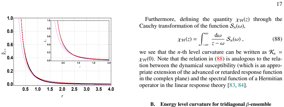
As can be seen, for higher values of β, ¯grr(r,β ) decays faster for large r, and its general behaviour is quite similar to the case of 2 × 2 rotationally invariant e ffective β ensemble studied next in section VII (see the plots in Figs. 9 and 10). 3 4 5 6 7 0.0000 0.0005 0.0010 0.0015 0.0020 0.0025 0.0030 r gr r 0.5 1.0 1.5 2.0 2.5 3.0 0.0 0.2 0.4 0.6 0...
Show all 101 references
-
[8]
The Ricci scalar corresponding to this two-dimensional ge- ometry changes from a constant to a non-constant value as the unitary symmetry of the GUE is broken
In sections III and V, we have studied in detail di fferent geometric quantities calculated from the QMTs corresponding to both a chaotic Hamiltonian (belonging to the GUE) and a Hamiltonian which shows a chaos-to-integrability transition. The Ricci scalar corresponding to thi...
-
[9]
Specifically, we have shown that the SFF, which controls the time-dependent part of the above-mentioned correlation function, is related to the FS
In section IV, we have discussed the procedure of ob- taining the FS (and the components of the QMT in general), from the connected correlation function involving theH term in the total Hamiltonian H = H0 + rH. Specifically, we have shown that the SFF, which controls the time-...
-
[10]
For a di fferent class of random matrix ensembles with a general Dyson index, and which shows a chaos-to- integrability transition, we have obtained the FS and showed that it diverges as one moves close to the integrable point. This is true for either of the ensembles, one of ...
-
[11]
As we have seen in section V, the Ricci scalar of the averaged QMT takes a generic parameter-dependent expres- sion compared to a fixed constant in the chaotic phase. Since the Ricci scalar being constant seems to be related to the fact that the GUE has rotational symmetry, it...
-
[12]
In this paper, we mostly consider the Gaussian weight function, i.e., potentials of the form V(H) = H2. However, one can consider more general weight functions, for which the ensemble would still retain the rotational invariance of the classical Gaussian ensembles (even though...
-
[13]
Finally, in this work, we have assumed that the Hamil- tonian governing the dynamics is Hermitian and consequently the ‘curvature’ of the parameter manifold is induced by the Hermitian inner product, which was reflected in the behaviour of the geometry in the integrability to ...
2023
-
[14]
− 1 2σ2 Tr(H2) r2 + 1 !# dH = 1 N2(r2 + 1) X m,n E
+ Tr( ˜H 2 1 ) # dH0 d ˜H1, (B1) where we have performed the trivial integration over ˜H2. Now performing two successive variable changes: first using H0 = H−r ˜H1 and subsequently ˜H1 = H1√ r2+1 + r r2+1 H, we can rewrite the above expression as,22 ¯grr(r) = 1 NZ(r2 + 1) X m,...
-
[15]
Furthermore, as in the case of ensembles discussed in sections VI and VII, the FS diverges in the limit r→ 0, i.e., as the Hamiltonian goes to the integrable phase
When the β = 2, the result matches with the expression in (58). Furthermore, as in the case of ensembles discussed in sections VI and VII, the FS diverges in the limit r→ 0, i.e., as the Hamiltonian goes to the integrable phase. 24
-
[16]
Bengtsson and K
I. Bengtsson and K. ˙Zyczkowski, Geometry of quantum states: an introduction to quantum entanglement (Cambridge univer- sity press, 2017)
2017
-
[17]
Chru ´sci´nski and A
D. Chru ´sci´nski and A. Jamiołkowski,Geometric phases in clas- sical and quantum mechanics (Springer, 2004)
2004
-
[18]
T. W. Kibble, Communications in Mathematical Physics 65, 189 (1979)
1979
-
[19]
Ashtekar and T
A. Ashtekar and T. A. Schilling, arXiv e-prints gr-qc /9706069 (1997), gr-qc/9706069
1997 arXiv
-
[20]
D. C. Brody and L. P. Hughston, Journal of Geometry and Physics 38, 19 (2001), quant-ph/9906086
2001 arXiv
-
[21]
Provost and G
J. Provost and G. Vallee, Communications in Mathematical Physics 76, 289 (1980)
1980
-
[22]
M. V . Berry, Proceedings of the Royal Society of London. A. Mathematical and Physical Sciences 392, 45 (1984)
1984
-
[23]
Simon, Phys
B. Simon, Phys. Rev. Lett. 51, 2167 (1983), URL https:// link.aps.org/doi/10.1103/PhysRevLett.51.2167
1983 doi
-
[24]
Zanardi, P
P. Zanardi, P. Giorda, and M. Cozzini, Phys. Rev. Lett. 99, 100603 (2007)
2007
-
[25]
You, Y .-W
W.-L. You, Y .-W. Li, and S.-J. Gu, Phys. Rev. E 76, 022101 (2007), URL https://link.aps.org/doi/10. 1103/PhysRevE.76.022101
2007
-
[26]
L. C. Venuti and P. Zanardi, Physical Review Letters 99, 095701 (2007)
2007
-
[27]
Kolodrubetz, V
M. Kolodrubetz, V . Gritsev, and A. Polkovnikov, Phys. Rev. B 88, 064304 (2013), URL https://link.aps.org/doi/10. 1103/PhysRevB.88.064304
2013
-
[28]
Kumar and T
P. Kumar and T. Sarkar, Phys. Rev. E 90, 042145 (2014), URL https://link.aps.org/doi/10.1103/PhysRevE.90. 042145
2014 doi
-
[29]
A. Dey, S. Mahapatra, P. Roy, and T. Sarkar, Phys. Rev. E 86, 031137 (2012), URL https://link.aps.org/doi/10. 1103/PhysRevE.86.031137
2012
-
[30]
Henriet, Phys
L. Henriet, Phys. Rev. B 97, 195138 (2018), URL https:// link.aps.org/doi/10.1103/PhysRevB.97.195138
2018 doi
-
[31]
Guti ´errez-Ruiz, J
D. Guti ´errez-Ruiz, J. Ch ´avez-Carlos, D. Gonzalez, J. G. Hirsch, and J. D. Vergara, Phys. Rev. B 105, 214106 (2022), URL https://link.aps.org/doi/10.1103/PhysRevB. 105.214106
2022 doi
-
[33]
Alexandrov and A
A. Alexandrov and A. Gorsky, Phys. Rev. E 107, 044211 (2023), URL https://link.aps.org/doi/10.1103/ PhysRevE.107.044211
2023
-
[34]
Xiao, M.-C
D. Xiao, M.-C. Chang, and Q. Niu, Rev. Mod. Phys. 82, 1959 (2010), URL https://link.aps.org/doi/10.1103/ RevModPhys.82.1959
2010
-
[36]
Mera and T
B. Mera and T. Ozawa, Phys. Rev. B 104, 045104 (2021), URL https://link.aps.org/doi/10.1103/PhysRevB.104. 045104
2021 doi
-
[37]
Het ´enyi and P
B. Het ´enyi and P. L ´evay, Phys. Rev. A 108, 032218 (2023), URL https://link.aps.org/doi/10.1103/PhysRevA. 108.032218
2023 doi
-
[38]
F. J. Dyson, Journal of Mathematical Physics 3, 1199 (1962)
1962
-
[39]
Bohigas, M.-J
O. Bohigas, M.-J. Giannoni, and C. Schmit, Physical review letters 52, 1 (1984)
1984
-
[40]
M. V . Berry, Proceedings of the Royal Society of London. A. Mathematical and Physical Sciences 400, 229 (1985)
1985
-
[41]
Bogomolny, U
E. Bogomolny, U. Gerland, and C. Schmit, Physical Review E 59, R1315 (1999)
1999
-
[42]
Robnik, Mathematics and Computers in Simulation 40, 159 (1996)
M. Robnik, Mathematics and Computers in Simulation 40, 159 (1996)
1996
-
[43]
Cheon, T
T. Cheon, T. Mizusaki, T. Shigehara, and N. Yoshinaga, Physi- cal Review A 44, R809 (1991)
1991
-
[45]
Lenz and F
G. Lenz and F. Haake, Physical review letters 67, 1 (1991)
1991
-
[46]
Shukla and A
P. Shukla and A. Pandey, Nonlinearity 10, 979 (1997)
1997
-
[47]
D. A. Rabson, B. N. Narozhny, and A. J. Millis, Phys. Rev. B 69, 054403 (2004), URL https://link.aps.org/doi/10. 1103/PhysRevB.69.054403
2004
-
[48]
Potters and J.-P
M. Potters and J.-P. Bouchaud, A First Course in Random Ma- trix Theory (Cambridge University Press, 2020)
2020
-
[49]
Mehta, Random Matrices (Academic Press, 1991), URL https://books.google.co.kr/books?id= vBHSAQAACAAJ
M. Mehta, Random Matrices (Academic Press, 1991), URL https://books.google.co.kr/books?id= vBHSAQAACAAJ
1991
-
[50]
Rosenzweig and C
N. Rosenzweig and C. E. Porter, Physical Review 120, 1698 (1960)
1960
-
[51]
Kravtsov, I
V . Kravtsov, I. Khaymovich, E. Cuevas, and M. Amini, New Journal of Physics 17, 122002 (2015)
2015
-
[52]
ˇCadeˇz, D
T. ˇCadeˇz, D. K. Nandy, D. Rosa, A. Andreanov, and B. Dietz, New Journal of Physics 26, 083018 (2024)
2024
-
[53]
Buijsman, Phys
W. Buijsman, Phys. Rev. B 109, 024205 (2024), URL https: //link.aps.org/doi/10.1103/PhysRevB.109.024205
2024 doi
-
[54]
De Tomasi and I
G. De Tomasi and I. M. Khaymovich, Phys. Rev. B 106, 094204 (2022), URL https://link.aps.org/doi/10. 1103/PhysRevB.106.094204
2022
-
[55]
von Soosten and S
P. von Soosten and S. Warzel, Letters in Mathematical Physics 109, 905 (2019)
2019
- [56]
-
[57]
Dumitriu and A
I. Dumitriu and A. Edelman, Journal of Mathematical Physics 43, 5830 (2002), ISSN 0022-2488, URL https://doi.org/ 10.1063/1.1507823
2002 doi
-
[58]
Buijsman, V
W. Buijsman, V . Cheianov, and V . Gritsev, Physical review let- ters 122, 180601 (2019)
2019
-
[59]
Sharipov, A
R. Sharipov, A. Tiutiakina, A. Gorsky, V . Gritsev, and A. Polkovnikov (2024), 2411.11968
2024 arXiv
-
[60]
Hauke, M
P. Hauke, M. Heyl, L. Tagliacozzo, and P. Zoller, Nature Physics 12, 778 (2016)
2016
-
[61]
Kolodrubetz, D
M. Kolodrubetz, D. Sels, P. Mehta, and A. Polkovnikov, Physics Reports 697, 1 (2017)
2017
-
[62]
You and L
W.-L. You and L. He, Journal of Physics: Condensed Matter 27, 205601 (2015)
2015
-
[63]
Br ´ezin and S
E. Br ´ezin and S. Hikami, Phys. Rev. E 55, 4067 (1997), URL https://link.aps.org/doi/10.1103/PhysRevE.55. 4067
1997 doi
-
[64]
Pechukas, Phys
P. Pechukas, Phys. Rev. Lett. 51, 943 (1983), URL https:// link.aps.org/doi/10.1103/PhysRevLett.51.943
1983 doi
-
[65]
Yukawa, Phys
T. Yukawa, Phys. Rev. Lett. 54, 1883 (1985), URL https:// link.aps.org/doi/10.1103/PhysRevLett.54.1883
1985 doi
-
[66]
Haake, Quantum Signatures of Chaos (Springer-Verlag Berlin, 2010)
F. Haake, Quantum Signatures of Chaos (Springer-Verlag Berlin, 2010)
2010
-
[67]
St ¨ockmann, Quantum Chaos (2007)
H.-J. St ¨ockmann, Quantum Chaos (2007)
2007
-
[68]
D. V . V oiculescu, K. J. Dykema, and A. Nica, Free random variables, vol. 1 (American Mathematical Soc., 1992)
1992
-
[69]
J. A. Mingo and R. Speicher, Free probability and random ma- trices, vol. 35 (Springer, 2017). 25
2017
-
[70]
Sierant, A
P. Sierant, A. Maksymov, M. Ku ´s, and J. Zakrzewski, Phys. Rev. E 99, 050102 (2019), URL https://link.aps.org/ doi/10.1103/PhysRevE.99.050102
2019 doi
-
[71]
Maksymov, P
A. Maksymov, P. Sierant, and J. Zakrzewski, Phys. Rev. B 99, 224202 (2019), URL https://link.aps.org/doi/10. 1103/PhysRevB.99.224202
2019
-
[72]
Penner, F
A.-G. Penner, F. von Oppen, G. Zarand, and M. R. Zirnbauer, Phys. Rev. Lett. 126, 200604 (2021), 2011.03557
2021 arXiv
-
[73]
Berry and P
M. Berry and P. Shukla, Journal of Physics A: Mathematical and Theoretical 53, 275202 (2020)
2020
-
[74]
P. N. Walker and M. Wilkinson, Phys. Rev. Lett. 74, 4055 (1995), URL https://link.aps.org/doi/10.1103/ PhysRevLett.74.4055
1995
-
[75]
E. J. Austin and M. Wilkinson, Nonlinearity 5, 1137 (1992)
1992
-
[76]
S. M. Carroll, Spacetime and geometry (Cambridge University Press, 2019)
2019
-
[77]
H. J. Lipkin, N. Meshkov, and A. J. Glick, Nucl. Phys. 62, 188 (1965)
1965
-
[78]
Meshkov, A
N. Meshkov, A. J. Glick, and H. J. Lipkin, Nucl. Phys. 62, 199 (1965)
1965
-
[79]
A. J. Glick, H. J. Lipkin, and N. Meshkov, Nucl. Phys. 62, 211 (1965)
1965
-
[80]
K. Pal, K. Pal, and T. Sarkar, Phys. Rev. E 107, 044130 (2023), URL https://link.aps.org/doi/10. 1103/PhysRevE.107.044130
2023
-
[81]
Kumar, S
P. Kumar, S. Mahapatra, P. Phukon, and T. Sarkar, Phys. Rev. E 86, 051117 (2012), URL https://link.aps.org/doi/10. 1103/PhysRevE.86.051117
2012
-
[82]
Cotler, N
J. Cotler, N. Hunter-Jones, J. Liu, and B. Yoshida, JHEP 11, 048 (2017), 1706.05400
2017 arXiv
-
[83]
J. S. Cotler, G. Gur-Ari, M. Hanada, J. Polchinski, P. Saad, S. H. Shenker, D. Stanford, A. Streicher, and M. Tezuka, JHEP 05, 118 (2017), [Erratum: JHEP 09, 002 (2018)], 1611.04650
2017 arXiv
- [84]
-
[85]
Livan, M
G. Livan, M. Novaes, and P. Vivo, Monograph Award 63, 914 (2018)
2018
-
[86]
Br ´ezin and A
E. Br ´ezin and A. Zee, Phys. Rev. E 49, 2588 (1994), URL https://link.aps.org/doi/10.1103/PhysRevE.49. 2588
1994 doi
-
[87]
M. V . Berry and M. Tabor, Proc. R. Soc. Lond. A 356, 375 (1977)
1977
-
[88]
Schierenberg, F
S. Schierenberg, F. Bruckmann, and T. Wettig, Phys. Rev. E 85, 061130 (2012), URL https://link.aps.org/doi/10. 1103/PhysRevE.85.061130
2012
-
[89]
T. H. Baker and P. J. Forrester, Communications in Mathemati- cal Physics 188, 175 (1997)
1997
-
[90]
Le Ca ¨er, C
G. Le Ca ¨er, C. Male, and R. Delannay, Physica A: Statistical Mechanics and its Applications 383, 190 (2007)
2007
-
[91]
Dumitriu and A
I. Dumitriu and A. Edelman, Journal of Mathematical Physics 47 (2006)
2006
-
[92]
Desrosiers and P
P. Desrosiers and P. J. Forrester, Nuclear Physics B 743, 307 (2006)
2006
-
[93]
P. J. Forrester, Log-gases and random matrices (LMS-34) (Princeton university press, 2010)
2010
-
[94]
A. K. Das and A. Ghosh, Physical Review E 105, 054121 (2022)
2022
-
[95]
B. N. Parlett, The symmetric eigenvalue problem(SIAM, 1998)
1998
-
[96]
Vivo and S
P. Vivo and S. N. Majumdar, Physica A: Statistical Mechanics and its Applications 387, 4839 (2008)
2008
-
[97]
Zakrzewski, Entropy 25, 491 (2023), 2302.05934
J. Zakrzewski, Entropy 25, 491 (2023), 2302.05934
2023 arXiv
-
[98]
Coleman, Introduction to many-body physics (Cambridge University Press, 2015)
P. Coleman, Introduction to many-body physics (Cambridge University Press, 2015)
2015
-
[99]
Altland and B
A. Altland and B. Simons, Condensed Matter Field Theory (Cambridge University Press, 2010)
2010
-
[100]
F. J. Dyson, Journal of Mathematical Physics 3, 1191 (1962)
1962
-
[101]
Nica and R
A. Nica and R. Speicher, Lectures on the combinatorics of free probability, vol. 13 (Cambridge University Press, 2006)
2006
-
[102]
Bellitti, S
M. Bellitti, S. Morampudi, and C. R. Laumann, Phys. Rev. B 100, 184201 (2019), 1908.02263
2019 arXiv
-
[103]
H. A. Camargo, Y . Fu, V . Jahnke, K. Pal, and K.-Y . Kim, arXiv e-prints arXiv:2503.20338 (2025), 2503.20338
2025
Reviewed August 6, 2026 · model on record in the stance chip above.
Discussion (0). Sign in to comment.