REVIEW 3 major objections 5 minor 62 references
An Empirical Bernstein Inequality for Dependent Data in Hilbert Spaces and Applications
T0 review · 3 major / 5 minor · reviewed 2026-08-06 · deepseek-v4-flash
Pith's one-line read This paper proves data-dependent Bernstein inequalities for bounded beta-mixing processes in a separable Hilbert space, in which the slow error term is governed by within-block correlation estimates rather than by the mixing time.
desk verdict A genuine empirical-Bernstein extension for beta-mixing Hilbert-valued processes; Theorems 1–3 look solid, but the practical guarantee leans on a mixing coefficient you have to guess, and Theorem 4 is less finished than the rest. read the letter →
The pith
A machine-rendered reading of the paper's core claim, the machinery that carries it, and where it could break.
The reading
What carries the argument
The carrying mechanism is the interlaced block decomposition plus empirical variance proxies. For $n=2m\tau$, the trajectory is split into two interlaced sequences of $m$ blocks of length $\tau$; Lemma 1 bounds the probability that the dependent sum exceeds a threshold by the sum of two independent block-sum probabilities plus $2(m-1)\beta_\mu(\tau)$. The variance proxies $\hat{V}_\tau(X)$ and $\check{V}_\tau(X)$ average inner products $\langle X_t,X_s\rangle$ over index pairs lying on the diagonal $\tau$-blocks $S_\tau$, with $\check{V}_\tau$ subtracting cross-block pairs to debias under stationarity. These proxies are fed into a vector Bernstein-type concentration inequality for independent block sums, derived from a bounded-difference inequality of McDiarmid, together with a separate concentration result that replaces expected variances by observed ones. The block size $\tau$ and the user-supplied mixing coefficient determine the effective number of blocks and the admissible failure probability.
What would settle it
Run many independent trajectories of a finite-state Markov chain with exactly computable $\beta$-mixing coefficients, set a failure level $\delta$, pick $\tau$ using the true $\beta_\mu(\tau)$ so that $\delta(\tau)>0$, and count how often Theorem 2's bound is violated; a violation frequency above $\delta$ would refute the inequality, while a simulation that first overestimates $\beta_\mu(\tau)$ by a little makes the failure condition $\delta(\tau)>0$ visibly fail.
Extended reading notes
Core claim
On the paper's own terms, the central discovery is that the deviation of an empirical mean from its expectation along a dependent trajectory is controlled, with probability at least $1-\delta$, by a data-dependent bound whose slow term shrinks with the temporal correlation within blocks of length $\tau$ rather than with the global mixing time. Specifically, Theorem 2 bounds $\|\frac{1}{n}\sum_i (X_i-\mathbb{E}[X_i])\|$ by $\sqrt{\frac{2\tau \hat{V}_\tau(X)}{n}(1+2\ln(4/\delta(\tau)))}+\frac{32\tau c}{3n}\ln(4/\delta(\tau))$, where $\hat{V}_\tau(X)$ is the average uncentered inner product over pairs separated by less than $\tau$ steps, and Theorem 3 gives a bias-corrected version $\check{V}_\tau(X)$ for stationary processes. The mixing coefficient $\beta_\mu(\tau)$ enters only through the log factors and through the positivity condition $\delta(\tau)=\delta-2(n/(2\tau)-1)\beta_\mu(\tau)>0$. The authors further derive a finite-sample risk bound for reduced-rank Koopman operator regression, and the paper's conclusion notes that the bounds are not yet adapted to exploit the effective dimension of the RKHS for minimax excess-risk rates.
Load-bearing premise
The user must know or correctly upper-bound the $\beta$-mixing coefficient $\beta_\mu(\tau)$ closely enough that $\delta(\tau)=\delta-2(n/(2\tau)-1)\beta_\mu(\tau)>0$; if the supplied coefficient is too small, the probability guarantee in every displayed bound disappears.
Editorial extensions
If this is right
- If within-block correlations decay quickly, the dominant error term for covariance estimation scales like $\sqrt{\hat{V}_\tau(X)\tau/n}$, which can be far smaller than the worst-case $O(1/\sqrt{n})$ term, giving nearly $O(1/n)$ behavior in the moderate-sample regime.
- The reduced-rank Koopman risk bound of Theorem 4 avoids the unverifiable regularity assumptions used in earlier operator-learning analyses and shows how ridge parameter, rank, and kernel correlations affect risk concentration at finite sample sizes.
- The same block-and-estimate argument extends to non-stationary trajectories, paying only an additive term quantifying the distance of the initial distribution from equilibrium.
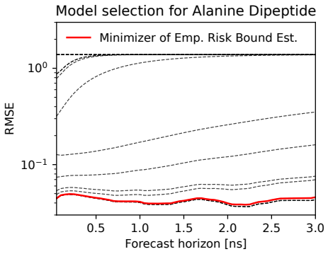
- Because the variance proxies are kernel-matrix quantities, the bounds are computable from the observed kernel matrix and can be minimized over model hyperparameters as a selection score, as illustrated on the molecular-dynamics example.
Reading between the lines
- The paper fixes $\tau$ from a plausibility-based $\beta_\mu(\tau)$; a testable extension would choose $\tau$ adaptively from the data by scanning the bound over admissible block sizes, which the experimental monotonicity in $\tau$ suggests may be stable.
- Comparing the biased and unbiased variance proxies on the same trajectory gives a data-only signal for how much nonstationarity degrades concentration, something the bounds themselves do not quantify but that their difference encodes.
- Connecting these empirical bounds to effective-dimension arguments, which the authors list as open, could turn the variance proxies into minimax-rate certificates for Koopman regression rather than only finite-sample upper bounds.
Editorial analysis
A structured set of objections, weighed in public.
Referee Report
Summary. The paper derives empirical Bernstein inequalities for bounded random variables taking values in a separable Hilbert space, under beta-mixing assumptions on the underlying process. The main results (Theorems 1-3) use Yu's block method to reduce dependent sums to independent block sums, with data-dependent variance proxies V_tau(X), e_Vtau(X), and b_Vtau(X). The paper applies these inequalities to covariance operator estimation in Hilbert-Schmidt norm and to risk bounds for reduced-rank regression of Koopman operators (Theorem 4). Numerical experiments cover covariance estimation from an Ornstein-Uhlenbeck process, a noisy ordered MNIST forecasting task, and model selection for alanine dipeptide dynamics.
Significance. If the stated results are correct, the paper is a useful contribution: it provides the first empirical Bernstein-type concentration inequalities for weakly dependent Hilbert-space-valued data, with variance terms that can be much smaller than worst-case bounds when temporal decorrelation is fast. The application to operator learning gives a non-asymptotic risk bound that avoids some unverifiable regularity assumptions used in prior work, and the authors provide an appendix with detailed proofs for Theorems 1-3 as well as publicly available code. The main weaknesses are that the probability guarantees are conditional on a user-supplied beta-mixing bound, that Theorem 1 appears to contain a constant-factor error in the linear term, and that the proof of Theorem 4 is only a sketch that relies on a nontrivial uniform argument over random norms.
major comments (3)
- [Section 2.2, Theorem 1; Appendix A.4] Theorem 1 assumes ||Xt|| <= c but bounds the deviation of (1/n) sum (Xt - E[Xt]). The centered variables Xt - E[Xt] are only bounded by 2c, not c. In the proof of Theorem 8 in Appendix A.4, the constant 8 tau c / (3n) is derived for mean-zero variables of norm at most c. Dropping the mean-zero assumption, as the text does, requires replacing c by 2c in the linear term, which would give 16 tau c / (3n) ln(2/delta(tau)). As written, Theorem 1's linear term is too small by a factor of two, and the proof does not explain why the smaller constant is valid.
- [Section 2.1 and Theorems 1-3] The stated probability guarantees are conditional on the condition delta(tau) = delta - 2(n/(2tau)-1) beta_mu(tau) > 0. Since beta_mu(tau) is not computable from a single trajectory for an unknown process, the user must supply an upper bound. The paper itself concedes in Section 2.1 that 'the coefficients beta_mu(tau) are fixed largely based on plausibility, making tau very uncertain.' If the supplied bound is too small, the displayed inequalities lose their probability status; if it is too large, the logarithmic factors grow and the advertised near-O(1/n) improvement disappears. The experiments use the analytically known OU mixing rate or an external eigenvalue estimate, so the regime in which beta must be guessed is not tested. The paper should either provide a sensitivity analysis for misspecified mixing coefficients or state clearly that the guarantee is conditional on the correctness of the mixing bound, not a fully data-driven 1-delta bound.
- [Appendix B.3, proof of Theorem 4] The proof of Theorem 4 is only a sketch and leaves a load-bearing gap. The events E(alpha1, alpha2, delta) are defined using Q(alpha1^{-1}, delta), but the monotonicity condition (ii) of Lemma 3 is not verified, and no formula for Q is given. More importantly, the condition bdelta_mu(tau, lambda) := 0.5 delta / ||bGr,lambda|| - 2(n/(2tau)-1) beta_mu(tau) > 0 contains the data-dependent random norm ||bGr,lambda||. The statement 'with probability at least 1-delta' is therefore not well-defined unless the probability of this random condition is controlled. The suggested substitution of delta/(2||bGr,lambda||) into the confidence parameter requires a uniform high-probability argument that is not supplied. This gap is central because Theorem 4 is one of the two advertised applications.
minor comments (5)
- [Section 3, covariance estimation] The sentence 'The transcription of the previous results fortunately, is affected by simply replacing all T= (1/n) sum_t E[phi(X_t) tensor phi(X_{t+1})] because the inner products change; ...' is garbled and should be rewritten.
- [Theorem 4 statement] Theorem 4 states 'Let delta >= 0', but a probability 'at least 1 - delta' requires 0 < delta < 1; the text should be corrected.
- [Figure 2 caption vs. text] The caption of Figure 2 says 'averaged over 50 independent simulations', while the main text in Section 4 says the plots have been averaged over 30 independent simulations; these numbers should be reconciled.
- [Section 2.3 proof sketch] The proof sketch refers to 'combining this with (2.3)', but equation (2.3) is not numbered anywhere; the reference should point to Proposition 1 in the appendix.
- [Appendix C.1.4] The notation 'K .2 = c^2 I_{n x n}' and similar expressions is unclear; it should be stated explicitly that this denotes the entrywise squared kernel matrix.
Circularity Check
No circular derivation: the paper's inequalities follow from external concentration results and Yu's block lemma, with the empirical variance estimates controlled by a union bound rather than identified with the target quantity.
full rationale
The main inequalities (Theorems 1-3) are proved by combining sufficiently general concentration inequalities for independent Hilbert-space vectors (Theorem 5, derived from Theorem 6, cited to McDiarmid and Pinelis-Sakhanenko) with Yu's block lemma (Lemma 1) and a union bound over the two interlaced block sequences. The data-dependent variance proxies eV_tau and bV_tau are not presupposed to equal V_tau; they are random quantities that Theorem 7, a published concentration inequality for empirical variance estimates, shows are within a penalty of the true variance with high probability. The probability guarantees of Theorems 1-3 are therefore derived, not definitional. Theorem 4's risk bound likewise conditions on high-probability estimates of empirical covariances and applies a standard uniform localization plus Tikhonov/Ivanov conversion (Lemma 3 and the cited equivalence in [27]); no displayed bound reduces to its own input. The genuinely fragile point is the user-supplied beta-mixing coefficient: the paper itself concedes in Section 2.1 that for an unknown process beta_mu(tau) is 'fixed largely based on plausibility, making tau very uncertain', and the required condition delta(tau) > 0 involves this uncomputable coefficient. That is a correctness or assumption risk, not circularity: the mixing coefficient is a stated input assumption, not a fitted parameter, and no theorem defines its conclusion in terms of that assumption. The self-citations ([31], [33], [27]) concern standard concentration and regularization-equivalence facts used as lemmas; they are independently published and are not used to assert uniqueness or to forbid alternatives. The derivation chain is thus self-contained against the quoted external results, and the appropriate circularity score is 0.
Assumptions & free parameters
assumptions (6)
- domain assumption The beta-mixing coefficient beta_mu(tau) is known or can be upper-bounded so that delta(tau) = delta - 2(n/(2tau)-1) beta_mu(tau) > 0.
- domain assumption The process is stationary for the improved estimator and for the operator-learning applications (Theorems 3, 4, 9).
- domain assumption Boundedness of the process: ||X_t|| <= c and ||phi(X_t)||^2 <= c_H almost surely.
- standard math Known concentration inequalities for independent variables: Theorems 6 and 7 from McDiarmid and Maurer-Pontil.
- standard math Yu's block method for beta-mixing processes (Lemma 2 and the interpolation argument).
- standard math Tikhonov-Ivanov equivalence for rank-constrained regression (Theorem 19 in [27]) and the event-sprinkling Lemma 3 from Anthony and Bartlett.
Cite this review
Pith. "Pith review of An Empirical Bernstein Inequality for Dependent Data in Hilbert Spaces and Applications." pith.science (2026). https://pith.science/paper/ZPAFPUGY
@misc{pith2026250707826,
  author       = {Pith},
  title        = {Pith review of: An Empirical Bernstein Inequality for Dependent Data in Hilbert Spaces and Applications},
  year         = {2026},
  howpublished = {\url{https://pith.science/paper/ZPAFPUGY}},
  note         = {Machine review of arXiv:2507.07826}
}
read the original abstract
Learning from non-independent and non-identically distributed data poses a persistent challenge in statistical learning. In this study, we introduce data-dependent Bernstein inequalities tailored for vector-valued processes in Hilbert space. Our inequalities apply to both stationary and non-stationary processes and exploit the potential rapid decay of correlations between temporally separated variables to improve estimation. We demonstrate the utility of these bounds by applying them to covariance operator estimation in the Hilbert-Schmidt norm and to operator learning in dynamical systems, achieving novel risk bounds. Finally, we perform numerical experiments to illustrate the practical implications of these bounds in both contexts.
Figures


Figures from the paper (9 more)


Reference graph
Works this paper leans on
-
[1]
Abeles, B., Clerico, E., and Neu, G. (2024). Generalization bounds for mixing processes via delayed online-to-pac conversions.arXiv preprint arXiv:2406.12600
work page Pith review arXiv 2024
-
[2]
Abélès, B., Clerico, E., and Neu, G. (2024). Online-to-pac generalization bounds under graph- mixing dependencies.arXiv preprint arXiv:2410.08977
work page Pith review arXiv 2024
-
[3]
Agarwal, A. and Duchi, J. C. (2012). The generalization ability of online algorithms for dependent data.IEEE Transactions on Information Theory, 59(1):573–587
work page 2012
-
[4]
Alquier, P., Doukhan, P., and Fan, X. (2019). Exponential inequalities for nonstationary markov chains.Dependence Modeling, 7(1):150–168
work page 2019
-
[5]
Anthony, M. M. and Bartlett, P. (1999).Learning in neural networks: theoretical foundations. Cambridge University Press
work page 1999
-
[6]
Audibert, J.-Y ., Munos, R., and Szepesvári, C. (2007). Variance estimates and exploration function in multi-armed bandit. InCERTIS Research Report 07–31. Citeseer
work page 2007
-
[7]
Audibert, J.-Y ., Munos, R., and Szepesvári, C. (2009). Exploration–exploitation tradeoff using variance estimates in multi-armed bandits.Theoretical Computer Science, 410(19):1876–1902
work page 2009
-
[8]
Blanchard, G. and Zadorozhnyi, O. (2019). Concentration of weakly dependent banach-valued sums and applications to statistical learning methods.Bernoulli, 25(4B):3421––3458
work page 2019
Show all 62 references
-
[9]
Bonati, L., Piccini, G., and Parrinello, M. (2021). Deep learning the slow modes for rare events sampling.Proceedings of the National Academy of Sciences, 118(44):e2113533118
2021
-
[10]
Bradley, R. C. (2005). Basic properties of strong mixing conditions. a survey and some open questions. 11
2005
-
[11]
L., Budiši´c, M., Kaiser, E., and Kutz, J
Brunton, S. L., Budiši´c, M., Kaiser, E., and Kutz, J. N. (2022). Modern Koopman Theory for Dynamical Systems.SIAM Review, 64(2):229–340
2022
-
[12]
A., Chapman, A
Burgess, M. A., Chapman, A. C., and Scott, P. (2020). An engineered empirical bernstein bound. InMachine Learning and Knowledge Discovery in Databases: European Conference, ECML PKDD 2019, Würzburg, Germany, September 16–20, 2019, Proceedings, Part III, pages 86–102. Springer
2020
-
[13]
and De Vito, E
Caponnetto, A. and De Vito, E. (2007). Optimal rates for the regularized least-squares algorithm. Foundations of Computational Mathematics, 7(3):331–368
2007
-
[14]
Chatterjee, S., Mukherjee, M., and Sethi, A. (2024). Generalization bounds for dependent data using online-to-batch conversion.arXiv preprint arXiv:2405.13666
2024 arXiv
-
[15]
and Kalmykov, Y
Coffey, W. and Kalmykov, Y . P. (2012).The Langevin equation: with applications to stochastic problems in physics, chemistry and electrical engineering, volume 27. World Scientific
2012
-
[16]
and Steinwart, I
Hang, H. and Steinwart, I. (2014). Fast learning from α-mixing observations.Journal of Multivariate Analysis, 127:184–199
2014
-
[17]
and Steinwart, I
Hang, H. and Steinwart, I. (2017). A bernstein-type inequality for some mixing processes and dynamical systems with an application to learning
2017
-
[18]
without
Jin, Y ., Ren, Z., Yang, Z., and Wang, Z. (2022). Policy learning" without”overlap: Pessimism and generalized empirical bernstein’s inequality.arXiv preprint arXiv:2212.09900
2022 arXiv
-
[19]
Kostic, V ., Inzerili, P., Lounici, K., Novelli, P., and Pontil, M. (2024a). Consistent long-term forecasting of ergodic dynamical systems. In2024 International Conference on Machine Learning
2024
-
[20]
Kostic, V ., Lounici, K., Novelli, P., and Pontil, M. (2023). Sharp spectral rates for koopman operator learning. In Oh, A., Naumann, T., Globerson, A., Saenko, K., Hardt, M., and Levine, S., editors,Advances in Neural Information Processing Systems, volume 36, pages 32328–323...
2023
-
[21]
Kostic, V ., Novelli, P., Maurer, A., Ciliberto, C., Rosasco, L., and Pontil, M. (2022). Learning dynamical systems via Koopman operator regression in reproducing kernel hilbert spaces. In Advances in Neural Information Processing Systems
2022
-
[22]
R., Lounici, K., Halconruy, H., Devergne, T., and Pontil, M
Kostic, V . R., Lounici, K., Halconruy, H., Devergne, T., and Pontil, M. (2024b). Learning the infinitesimal generator of stochastic diffusion processes.arXiv preprint arXiv:2405.12940
2024 arXiv
-
[23]
R., Novelli, P., Grazzi, R., Lounici, K., and Pontil, M
Kostic, V . R., Novelli, P., Grazzi, R., Lounici, K., and Pontil, M. (2024c). Learning invariant representations of time-homogeneous stochastic dynamical systems. InICLR 2024
2024
-
[24]
Levin, D. A. and Peres, Y . (2017).Markov chains and mixing times, volume 107. American Mathematical Soc
2017
-
[25]
Li, Z., Meunier, D., Mollenhauer, M., and Gretton, A. (2022). Optimal rates for regularized conditional mean embedding learning. InAdvances in Neural Information Processing Systems
2022
-
[26]
and Austern, M
Liu, T. and Austern, M. (2023). Wasserstein-p bounds in the central limit theorem under local dependence.Electronic Journal of Probability, 28:1–47
2023
-
[27]
Luise, G., Stamos, D., Pontil, M., and Ciliberto, C. (2019). Leveraging low-rank relations between surrogate tasks in structured prediction. InInternational Conference on Machine Learning, pages 4193–4202. PMLR
2019
-
[28]
Majda, A. J. and Harlim, J. (2012).Filtering complex turbulent systems. Cambridge University Press
2012
-
[29]
(1952).Portfolio selection, volume 7
Markowitz, H. (1952).Portfolio selection, volume 7. Wiley Online Library
1952
-
[30]
and Ramdas, A
Martinez-Taboada, D. and Ramdas, A. (2024). Empirical bernstein in smooth banach spaces. arXiv preprint arXiv:2409.06060. 12
2024 arXiv
-
[31]
Maurer, A. (2012). Thermodynamics and concentration.Bernoulli, 18(2):434–454
2012
-
[32]
and Pontil, M
Maurer, A. and Pontil, M. (2009). Empirical bernstein bounds and sample variance penalization. arXiv preprint arXiv:0907.3740
2009 arXiv
-
[33]
and Pontil, M
Maurer, A. and Pontil, M. (2018). Empirical bounds for functions with weak interactions. In Conference On Learning Theory, pages 987–1010. PMLR
2018
-
[34]
McDiarmid, C. (1998). Concentration. InProbabilistic Methods of Algorithmic Discrete Mathematics, pages 195–248, Berlin. Springer
1998
-
[35]
Meir, R. (2000). Nonparametric time series prediction through adaptive model selection. Machine learning, 39:5–34
2000
-
[36]
Modha, D. S. and Masry, E. (1996). Minimum complexity regression estimation with weakly dependent observations.IEEE Transactions on Information Theory, 42(6):2133–2145
1996
-
[37]
and Rostamizadeh, A
Mohri, M. and Rostamizadeh, A. (2008). Rademacher complexity bounds for non-iid processes. Advances in Neural Information Processing Systems, 21
2008
-
[38]
Mollenhauer, M., Klus, S., Schütte, C., and Koltai, P. (2022). Kernel autocovariance operators of stationary processes: Estimation and convergence.Journal of Machine Learning Research, 23(327):1–34
2022
-
[39]
Oneto, L., Ridella, S., and Anguita, D. (2016). Tikhonov, ivanov and morozov regularization for support vector machine learning.Machine Learning, 103:103–136
2016
-
[40]
Pavliotis, G. A. (2014).Stochastic Processes and Applications. Springer New York
2014
-
[41]
Peel, T., Anthoine, S., and Ralaivola, L. (2010). Empirical bernstein inequalities for u-statistics. InNeural Information Processing Systems (NIPS), number 23, pages 1903–1911
2010
-
[42]
Peel, T., Anthoine, S., and Ralaivola, L. (2013). Empirical bernstein inequality for martingales: Application to online learning
2013
-
[43]
M., Schaller, M., Worthmann, K., Peitz, S., and Nüske, F
Philipp, F. M., Schaller, M., Worthmann, K., Peitz, S., and Nüske, F. (2024). Error bounds for kernel-based approximations of the koopman operator.Applied and Computational Harmonic Analysis, 71:101657
2024
-
[44]
A., Savtchenko, L
Rusakov, D. A., Savtchenko, L. P., and Latham, P. E. (2020). Noisy synaptic conductance: bug or a feature?Trends in Neurosciences, 43(6):363–372
2020
-
[45]
and Strimmer, K
Schäfer, J. and Strimmer, K. (2005). A shrinkage approach to large-scale covariance matrix estimation and implications for functional genomics.Statistical Applications in Genetics and Molecular Biology, 4(1):Article 32
2005
-
[46]
Schug, S., Benzing, F., and Steger, A. (2021). Presynaptic stochasticity improves energy efficiency and helps alleviate the stability-plasticity dilemma.Elife, 10:e69884
2021
-
[47]
and Kontorovich, A
Shalizi, C. and Kontorovich, A. (2013). Predictive pac learning and process decompositions. Advances in neural information processing systems, 26
2013
-
[48]
and Jebara, T
Shivaswamy, P. and Jebara, T. (2010). Empirical bernstein boosting. InProceedings of the Thirteenth International Conference on Artificial Intelligence and Statistics, pages 733–740. JMLR Workshop and Conference Proceedings
2010
-
[49]
and Zhou, D.-X
Smale, S. and Zhou, D.-X. (2009). Online learning with markov sampling.Analysis and Applications, 7(01):87–113
2009
-
[50]
and Christmann, A
Steinwart, I. and Christmann, A. (2009). Fast learning from non-iid observations.Advances in neural information processing systems, 22
2009
-
[51]
Steinwart, I., Hush, D., and Scovel, C. (2009). Learning from dependent observations.Journal of Multivariate Analysis, 100(1):175–194. 13
2009
-
[52]
(2003).Financial modelling with jump processes
Tankov, P. (2003).Financial modelling with jump processes. Chapman and Hall/CRC
2003
-
[53]
Tolstikhin, I. O. and Seldin, Y . (2013). Pac-bayes-empirical-bernstein inequality.Advances in Neural Information Processing Systems, 26
2013
-
[54]
Tuckerman, M. E. (2023).Statistical Mechanics: Theory and Molecular Simulation. Oxford university press
2023
-
[55]
and Navarra, A
von Storch, H. and Navarra, A. (1999). Principal oscillation patterns: A review.Journal of Climate, 12(12):3519–3535
1999
-
[56]
and Ramdas, A
Waudby-Smith, I. and Ramdas, A. (2024). Estimating means of bounded random variables by betting.Journal of the Royal Statistical Society Series B: Statistical Methodology, 86(1):1–27
2024
-
[57]
and Noé, F
Wehmeyer, C. and Noé, F. (2018). Time-lagged autoencoders: Deep learning of slow collective variables for molecular kinetics.The Journal of chemical physics, 148(24)
2018
-
[58]
Yu, B. (1994). Rates of convergence for empirical processes of stationary mixing sequences. The Annals of Probability, pages 94–116
1994
-
[59]
maximal sum of conditional variances
Ziemann, I., Tu, S., Pappas, G. J., and Matni, N. (2024). The noise level in linear regression with dependent data.Advances in Neural Information Processing Systems, 36. 14 Supplementary Material A Hilbert space-valued concentration for dependent, non-stationary sequences. Fir...
2024
-
[60]
If we drop the mean-zero assumption, this becomes Theorem 1
-
[61]
To interpret the first term on the right-hand side, note the similarity to the variance of P Xt, which would be E X Xt 2 = X (t,s)∈[T]×[T] E[⟨X t, Xs⟩]
-
[62]
In the proof above, the functionsF(X)andF ′ (X)were constants
If the Xt are independent, we can set τ= 1 and βX (τ) = 0, and we recover Theorem 5 up to a constant factor of √ 2on the first, and2on the second term. In the proof above, the functionsF(X)andF ′ (X)were constants. But let F(X) = vuut mX k=1 X i∈Ik Xi 2 1+ p 2 ln (4/δ) + 16cτ ...
Reviewed August 6, 2026 · model on record in the stance chip above.
Discussion (0). Sign in to comment.