REVIEW 3 major objections 6 minor 53 references
A Novel and Simple Invariant-Domain-Preserving Framework for PAMPA Scheme: 1D Case
T0 review · 3 major / 6 minor · reviewed 2026-08-11 · deepseek-v4-flash
Pith's one-line read The paper proves that a single local scaling limiter on cell midpoint values, together with an invariant-domain-preserving numerical flux, keeps updated cell averages of the PAMPA scheme inside the convex invariant domain under a CFL…
desk verdict A genuinely useful IDP framework for PAMPA with a clean cell-average theorem; the scalar point-value reformulation has an unexamined non-injective regime that should be fixed before publication. read the letter →
The pith
A machine-rendered reading of the paper's core claim, the machinery that carries it, and where it could break.
The reading
What carries the argument
The load-bearing object is the cell average decomposition (CAD) together with the automatic IDP reformulation of the non-conservative point-value equations. The CAD rewrites the cell average as the weighted sum $(1/6, 4/6, 1/6)$ of limited endpoint values and the midpoint value, so the PAMPA average update separates into a convex combination of two first-order IDP fluxes, each evaluated on a time step $6\Delta t$; Theorem 5.1 then follows from convexity of $G$ and the IDP property of the numerical flux. The point-value machinery is a change of variables $W = \Psi(U)$ chosen so that $\Psi^{-1}(\mathbb{R}^d) \subseteq G$, using Softplus-type and Clipped ReLU maps; the point-value evolution then keeps $U$ in $G$ for every real $W$ without any limiter.
What would settle it
Take a smooth scalar problem with initial data strictly inside [Umin, Umax], run the point-value scheme in a regime where the reconstructed transformed variable w enters the clipped region (w < 0 or w > 1), and compare with the exact solution on successive mesh refinements; if convergence order drops below three or the numerical solution approaches the wrong limit in that regime, the claim that the automatic IDP reformulation is a consistent high-order point-value scheme fails.
Extended reading notes
Core claim
The central discovery is that the PAMPA update for cell averages can be decomposed as a convex combination of a midpoint value and two first-order invariant-domain-preserving steps, provided the cell average decomposition (CAD) $\bar{U}_{j+1/2} = \frac{1}{6} U_j^R + \frac{4}{6} U_{j+1/2} + \frac{1}{6} U_{j+1}^L$ is preserved. A local scaling limiter is applied to midpoint values, and the cell-interface endpoint values are adjusted accordingly so that the CAD survives; then Theorem 5.1 says the updated cell average stays in $G$ whenever $\lambda_{\max} \Delta t / \Delta x \le 1/6$ and the numerical flux is IDP. The point-value evolution is made unconditionally bound-preserving by choosing variables $W = \Psi(U)$ whose inverse map sends all real vectors into $G$: for the Euler equations, $q = \ln(e^{\rho/\rho_{\mathrm{ref}}} - 1)$, velocity, and specific entropy; for scalar laws, $u = U_{\min} + (U_{\max} - U_{\min}) \min\{\mathrm{ReLU}(w), 1\}$. Because the updated $W$ is any real vector, $U = \Psi^{-1}(W)$ always lies in $G$.
Load-bearing premise
The scheme's point-value accuracy rests on the transformed variables W remaining a faithful parametrization of the physical state even where the bound-enforcing maps (clipped ReLU in the scalar case and the softplus density transform) are not one-to-one; the paper does not analyze that clipped non-injective regime or prove third-order accuracy there.
Editorial extensions
If this is right
- If Theorem 5.1 holds for general systems, third-order PAMPA cell averages can be made invariant-domain-preserving by a simple midpoint limiter and an IDP numerical flux, at CFL $\le 1/6$, with no convex blending of high- and low-order solutions.
- For the Euler and MHD equations, the Softplus/entropy variable set turns positivity of density and pressure into a built-in property of the point-value evolution, so no post-step positivity fix is needed.
- The scheme retains third-order accuracy in smooth tests even with the IDP limiter and the oscillation-control techniques, as the convergence tables demonstrate.
- The same construction applies to scalar conservation laws with any interval invariant domain via the clipped ReLU mapping.
- Because the proof relies only on convexity and the IDP property of the numerical flux, the framework extends directly to higher-order SSP time discretizations, which are convex combinations of forward Euler steps.
Reading between the lines
- This framework would likely carry over to any element-based method whose cell average can be expressed as a convex combination of nodal or midpoint values, so analogous IDP cell-average updates could be built for unstructured or arbitrary-order variants of PAMPA.
- The clipped non-injective regime of the scalar mapping (w outside [0,1]) remains unanalyzed; a natural next step is to test whether the point-value scheme stays third-order accurate and consistent there, or whether a refined mapping is needed.
- The paper's invariant domains are positivity and maximum-principle sets; adding an entropy constraint would require a wider admissible set or larger wave-speed estimates, and the automatic IDP reformulation would need to be rechecked in that setting.
Editorial analysis
A structured set of objections, weighed in public.
Referee Report
Summary. The paper develops an invariant-domain-preserving (IDP) framework for the 1D PAMPA scheme. It first analyzes the original PAMPA cell-average update through a cell-average decomposition, showing that midpoint values must lie in the invariant domain for the continuous-flux update to preserve the domain. It then introduces a local scaling limiter for midpoint values and, using an IDP numerical flux, proves in Theorem 5.1 that the resulting cell-average update preserves the invariant domain under a CFL condition without additional convex limiting. For point values, the paper proposes non-conservative reformulations in transformed variables: a Softplus-type density/entropy mapping for the Euler and MHD systems, and a clipped ReLU mapping for scalar conservation laws, claiming an unconditionally limiter-free IDP point-value scheme. Oscillation-eliminating and monotonicity-preserving techniques are added, and numerical experiments on advection, Burgers, Euler, and MHD equations demonstrate accuracy and robustness.
Significance. The cell-average IDP theorem is clean and useful: the local midpoint limiter preserves the crucial cell-average decomposition, and the CFL condition λ_max Δt/Δx ≤ 1/6 is explicit and simple. The Euler/MHD variable transformation q = ln(e^{ρ/ρ_ref} − 1) is a genuinely elegant way to enforce positivity of density and pressure by construction, and the numerical tests include very demanding problems such as the double rarefaction, Leblanc, and strong-field MHD cases. If the scalar point-value gap discussed below is resolved, the framework would be a valuable contribution to bound-preserving PAMPA schemes. The main reservation is that the scalar point-value IDP claim relies on a non-injective clipped mapping whose consistency with the original conservation law is not analyzed, and the accuracy tests do not exercise the saturated regime of that mapping.
major comments (3)
- [Section 5.3, Eq. (5.17)] The scalar point-value IDP property is enforced by the non-injective mapping u = (Umax-Umin) min{ReLU(w),1} + Umin. For w < 0 or w > 1, the inverse Ψ^{-1}(w) is constant, so the associated non-conservative equation w_t + f'(Ψ^{-1}(w)) w_x = 0 is not equivalent to the original conservation law, and the update (5.18) is not shown to be a consistent discretization in the saturated regime. The IDP property is guaranteed by construction, but correctness as a method for the conservation law is not. The convergence tests in Section 7.1 use u0 = 1 + sin^4(2πx) with G = [1,2], so they do not demonstrate accuracy when clipping is active in smooth regions. Please either provide an analysis of the saturated regime, add a test where w leaves [0,1] in a smooth region and verify the scheme remains consistent, or explicitly qualify the claim as applying only when the mapping is injective.
- [Section 5.1, Eqs. (5.4)-(5.7)] The formulas for θρ and θp appear to use the endpoint value U^n_j rather than the cell average \bar U^n_{j+1/2} as the reference state: θρ is written with ρ^n_j, and θp with p(U^n_j). As written, the limited midpoint value is not guaranteed to lie in G, and the cell-average decomposition (5.8), which is essential for Theorem 5.1, is not guaranteed. If this is a typographical error and the cell average \bar U^n_{j+1/2} is intended, please correct the notation; otherwise the proof of Theorem 5.1 is incomplete.
- [Section 5.2, Theorem 5.1] The theorem is stated for general hyperbolic systems, but the proof relies on the existence of an 'IDP numerical flux' satisfying (5.10) with a specified CFL constant c0. For the local Lax-Friedrichs flux used in the experiments, this property is not automatic for arbitrary invariant domains; it depends on the generalized Lax-Friedrichs splitting property (2.9) with the chosen wave-speed estimate. The hypothesis should be stated explicitly so that the theorem's applicability to the Euler and MHD systems is precise.
minor comments (6)
- [Section 5.3] The text says 'For the scalar conservation law (2.5)' but equation (2.5) is the Euler invariant domain; the scalar maximum principle is (2.3). Please correct the cross-reference.
- [Tables 1 and 2] Several entries omit the exponent marker, e.g., '1.09-4' and '1.65-6' should be '1.09e-4' and '1.65e-6'. These typos make the tables harder to read.
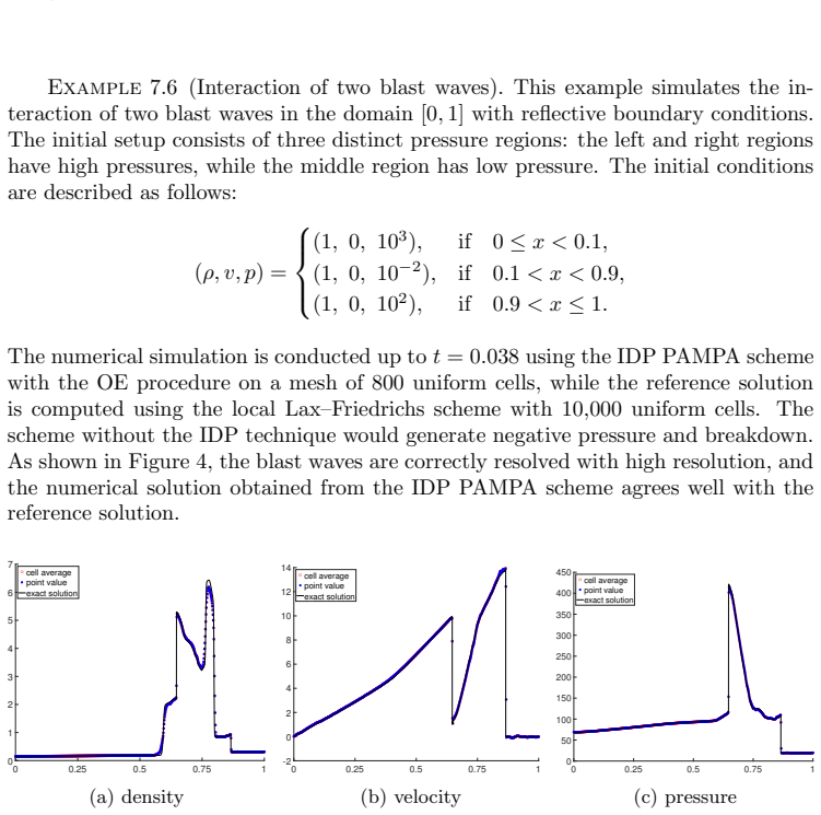
- [Figures 4 and 6] The captions label the compared curve as 'exact solution', but the text describes it as a reference solution computed on a very fine mesh. Please relabel the reference curves for accuracy.
- [Section 6.1] The OE procedure is described using a scalar quantity p, and it is not immediately clear how it is applied to systems of conservation laws or to the transformed variables W. Please clarify the component-wise or variable-wise application and state what happens when S_R = S_L.
- [Section 5.3] The phrase 'unconditionally limiter-free IDP scheme for point values' may be misleading, because the point-value update in (5.16) still uses the midpoint values modified by the Step 1 local scaling limiter. The absence of a post-update limiter on point values should be stated more precisely.
- [References] Reference [4] lists the arXiv URL twice; please remove the duplicated URL.
Circularity Check
Point-value IDP is self-definitional via the variable mapping; the cell-average IDP theorem is an independent, non-circular derivation.
-
self definitional
[Section 5.3, Eqs. (5.14)–(5.18), especially Eq. (5.17)]
"Typically, we can find a suitable set of variables W, such that the range of the mapping W = Ψ(U) is Rd, i.e, Ψ(G) = Rd. In the words, for any W ∈ Rd, we always have U = Ψ−1(W) ∈ G. This automatically ensures the IDP property of the point values. ... This mapping ensures that, for any w ∈ R, we always have u ∈ [Umin, Umax]."
The 'unconditionally limiter-free IDP' property for point values is not a consequence of the numerical residuals Φ or of any CFL condition; it follows immediately from the definition of Ψ−1, whose range is G by construction. Since U^{n+1}_j = Ψ−1(W^{n+1}_j), every possible value of W^{n+1}_j maps into G, so the claimed invariant-domain preservation reduces to the choice of the variable transformation. The scalar formula (5.17) makes this explicit: the clipped ReLU map has range [Umin,Umax] by definition. The same construction is used for Euler/MHD via the Softplus-type variables in (5.14). Thus the point-value IDP claim is self-definitional rather than a derived property of the scheme dynamics.
full rationale
The cell-average IDP theorem (Theorem 5.1) is self-contained: it combines the local scaling IDP limiter, the cell-average decomposition (5.8), and the standard notion of an IDP numerical flux (5.10), and the convex-combination proof is a genuine derivation independent of the variable-mapping construction. The generalized Lax–Friedrichs splitting property and wave-speed estimates cited from [46,41] are external mathematical facts, not fitted inputs, and they are not used to define the target IDP result. No fitted parameter is renamed as a prediction. The only circular-like element is the point-value IDP claim in Section 5.3, which is guaranteed by design through the range of the mapping Ψ−1 rather than by the numerical evolution; the paper is transparent about this ('automatically ensures'). The separate non-injectivity issue of the scalar map (5.17) in the clipped region is a consistency/correctness gap for the W-evolution, not an additional circularity. Overall the circularity is mild and partial, with the main provable cell-average result retaining independent content.
Assumptions & free parameters
free parameters (3)
- Reference density rho_ref in softplus map =
1
- Positivity floors epsilon_rho, epsilon_p in system limiter =
10^-13 (with min over cell averages)
- MP limiter constants alpha, beta =
2, 4
assumptions (4)
- domain assumption The invariant domains for scalar, Euler, and MHD equations are convex and satisfy the generalized LF splitting property (2.9) with the stated lambda_max.
- standard math The chosen numerical flux Fhat is IDP in the sense of (5.10) under suitable CFL conditions.
- ad hoc to paper The mapping Psi^{-1} maps all of R^d into the invariant domain G for the softplus/ReLU variables.
- standard math SSP time discretizations are convex combinations of forward Euler steps.
invented entities (1)
-
Softplus/ReLU-based variable transformation W = Psi(U) for Euler and scalar equations
Cite this review
Pith. "Pith review of A Novel and Simple Invariant-Domain-Preserving Framework for PAMPA Scheme: 1D Case." pith.science (2026). https://pith.science/paper/ZZSN3Y2F
@misc{pith2026241203423,
  author       = {Pith},
  title        = {Pith review of: A Novel and Simple Invariant-Domain-Preserving Framework for PAMPA Scheme: 1D Case},
  year         = {2026},
  howpublished = {\url{https://pith.science/paper/ZZSN3Y2F}},
  note         = {Machine review of arXiv:2412.03423}
}
read the original abstract
The PAMPA (Point-Average-Moment PolynomiAl-interpreted) method, proposed in [R. Abgrall, Commun. Appl. Math. Comput., 5: 370-402, 2023], combines conservative and non-conservative formulations of hyperbolic conservation laws to evolve cell averages and point values. Solutions to hyperbolic conservation laws typically have an invariant domain, and ensuring numerical solutions stay within this domain is essential yet nontrivial. This paper presents a novel framework for designing efficient Invariant-Domain-Preserving (IDP) PAMPA schemes. We first analyze the IDP property for updated cell averages in the original PAMPA scheme, revealing the role of cell average decomposition and midpoint values in maintaining the invariant domain. This analysis highlights the difficulty of relying on continuous fluxes alone to preserve the invariant domain. Building on these insights, we introduce a simple IDP limiter for cell midpoint values, and propose a provably IDP PAMPA scheme that guarantees the preservation of the invariant domain for updated cell averages without requiring post-processing limiters. This approach contrasts with existing bound-preserving PAMPA schemes, which often require additional convex limiting to blend high-order and low-order solutions. Most notably, inspired by the Softplus and Clipped ReLU functions from machine learning, we propose an automatic IDP reformulation of the governing equations, resulting in an unconditionally limiter-free IDP scheme for evolving point values. We also introduce techniques to suppress spurious oscillations, enabling the scheme to capture strong shocks effectively. Numerical experiments on 1D problems, including the linear convection equation, Burgers equation, the compressible Euler equations, and MHD equations, demonstrate the accuracy and robustness of the proposed IDP PAMPA scheme.
Figures


Figures from the paper (7 more)


Reference graph
Works this paper leans on
-
[1]
R. Abgrall, A combination of residual distribution and the active flux formulations or a new class of schemes that can combine several writings of the same hyperbolic problem: application to the 1D Euler equations, Communications on Applied Mathematics and Com- putation, 5 (2023), pp. 370–402
work page 2023
-
[2]
R. Abgrall and W. Barsukow, Extensions of active flux to arbitrary order of accuracy , ESAIM, Math. Model. Numer. Anal., 57 (2023), pp. 991–1027
work page 2023
-
[3]
R. Abgrall and W. Barsukow, A hybrid finite element–finite volume method for conservation laws, Applied Mathematics and Computation, 447 (2023), p. 127846
work page 2023
-
[4]
R. Abgrall, M. Jiao, Y. Liu, and K. Wu , Bound-preserving point-average-moment polynomial-interpreted (PAMPA) scheme: One-dimensional case , arXiv preprint, 2410.14292 (2024), https://arxiv.org/abs/2410.14292, https://arxiv.org/abs/2410.14292
arXiv 2024
-
[5]
R. Abgrall, J. Lin, and Y. Liu, Active flux for triangular meshes for compressible flows problems, Beijing Journal of Pure and Applied Mathematics, (in press). also Arxiv preprint 2312.11271
-
[6]
R. Abgrall and Y. Liu, A new approach for designing well-balanced schemes for the shallow water equations: A combination of conservative and primitive formulations , SIAM Journal on Scientific Computing, 46 (2024), pp. A3375–A3400
work page 2024
-
[7]
W. Barsukow, The active flux scheme for nonlinear problems, Journal of Scientific Computing, 86 (2020), p. 3
work page 2020
-
[8]
W. Barsukow and J. P. Berberich, A well-balanced active flux method for the shallow water equations with wetting and drying , Communications on Applied Mathematics and Compu- tation, 6 (2024), pp. 2385–2430
work page 2024
Show all 53 references
-
[9]
Barsukow, J
W. Barsukow, J. Hohm, C. Klingenberg, and P. L. Roe, The active flux scheme on Carte- sian grids and its low mach number limit , Journal of Scientific Computing, 81 (2019), IDP FRAMEWORK FOR PAMPA 27 pp. 594–622
2019
-
[10]
Calhoun, E
D. Calhoun, E. Chudzik, and C. Helzel, The Cartesian grid Active Flux method with adaptive mesh refinement , Journal of Scientific Computing, 94 (2023), p. 54
2023
-
[11]
Chudzik, C
E. Chudzik, C. Helzel, and D. Kerkmann, The Cartesian grid active flux method: Lin- ear stability and bound preserving limiting , Applied Mathematics and Computation, 393 (2021), p. 125501
2021
-
[12]
Cockburn, S.-Y
B. Cockburn, S.-Y. Lin, and C.-W. Shu, TVB Runge-Kutta local projection discontinuous Galerkin finite element method for conservation laws III: One-dimensional systems , Jour- nal of Computational Physics, 84 (1989), pp. 90–113
1989
-
[13]
Cockburn and C.-W
B. Cockburn and C.-W. Shu, The Runge–Kutta discontinuous Galerkin method for conser- vation laws V: Multidimensional systems , Journal of Computational Physics, 141 (1998), pp. 199–224
1998
-
[14]
S. Cui, S. Ding, and K. Wu, Is the classic convex decomposition optimal for bound-preserving schemes in multiple dimensions?, Journal of Computational Physics, 476 (2023), p. 111882
2023
-
[15]
S. Cui, S. Ding, and K. Wu, On optimal cell average decomposition for high-order bound- preserving schemes of hyperbolic conservation laws , SIAM Journal on Numerical Analysis, 62 (2024), pp. 775–810
2024
-
[16]
J. Duan, W. Barsukow, and C. Klingenberg, Active flux methods for hyperbolic conser- vation laws–flux vector splitting and bound-preservation , arXiv preprint arXiv:2411.00065, (2024)
2024 arXiv
-
[17]
Eymann and P
T. Eymann and P. Roe, Active flux schemes , in 49th AIAA Aerospace Sciences Meeting including the New Horizons Forum and Aerospace Exposition, Orlando,Florida, Jan. 2011
2011
-
[18]
Eymann and P
T. Eymann and P. Roe, Active flux schemes for systems , in 20th AIAA Computational Fluid Dynamics Conference, American Institute of Aeronautics and Astronautics, June 2011
2011
-
[19]
T. A. Eymann and P. L. Roe, Multidimensional active flux schemes , in 21st AIAA Compu- tational Fluid Dynamics Conference, American Institute of Aeronautics and Astronautics, June 2013
2013
-
[20]
F an and P
D. F an and P. L. Roe, Investigations of a new scheme for wave propagation , in 22nd AIAA Computational Fluid Dynamics Conference, American Institute of Aeronautics and Astro- nautics, 2015
2015
-
[21]
Guermond, M
J.-L. Guermond, M. Nazarov, B. Popov, and I. Tomas, Second-order invariant domain preserving approximation of the Euler equations using convex limiting , SIAM Journal on Scientific Computing, 40 (2018), pp. A3211–A3239
2018
-
[22]
Guermond and B
J.-L. Guermond and B. Popov, Fast estimation from above of the maximum wave speed in the Riemann problem for the Euler equations , J. Comput. Phys., 321 (2016), pp. 908–926, https://doi.org/10.1016/j.jcp.2016.05.054
2016 doi
-
[23]
Guermond and B
J.-L. Guermond and B. Popov, Invariant domains and second-order continuous finite element approximation for scalar conservation equations, SIAM Journal on Numerical Analysis, 55 (2017), pp. 3120–3146
2017
-
[24]
Harten, B
A. Harten, B. Engquist, S. Osher, and S. R. Chakravarthy, Uniformly high order accurate essentially non-oscillatory schemes, III , Journal of Computational Physics, 71 (1987), pp. 231–303
1987
-
[25]
Helzel, D
C. Helzel, D. Kerkmann, and L. Scandurra, A new ADER method inspired by the active flux method, Journal of Scientific Computing, 80 (2019), pp. 1463–1497
2019
-
[26]
X. Y. Hu, N. A. Adams, and C.-W. Shu, Positivity-preserving method for high-order conser- vative schemes solving compressible Euler equations , Journal of Computational Physics, 242 (2013), pp. 169–180
2013
-
[27]
V. P. Korobeinikov, Problems of point blast theory, Springer Science & Business Media, 1991
1991
-
[28]
D. Kuzmin, Monolithic convex limiting for continuous finite element discretizations of hyper- bolic conservation laws , Computer Methods in Applied Mechanics and Engineering, 361 (2020), p. 112804
2020
-
[29]
Kuzmin, M
D. Kuzmin, M. Quezada de Luna, D. I. Ketcheson, and J. Gr¨ull, Bound-preserving flux limiting for high-order explicit Runge–Kutta time discretizations of hyperbolic conservation laws, J. Sci. Comput., 91 (2022)
2022
-
[30]
Liang and Z
C. Liang and Z. Xu, Parametrized maximum principle preserving flux limiters for high order schemes solving multi-dimensional scalar hyperbolic conservation laws, Journal of Scientific Computing, 58 (2014), pp. 41–60
2014
-
[31]
X.-D. Liu, S. Osher, and T. Chan, Weighted essentially non-oscillatory schemes , Journal of Computational Physics, 115 (1994), pp. 200–212
1994
-
[32]
Y. Liu, Well-balanced point-average-moment polynomial-interpreted (PAMPA) methods for shallow water equations on triangular meshes , arXiv preprint, 2409.12606 (2024), https: //arxiv.org/abs/2409.12606. 28 R´EMI ABGRALL, MIAOSEN JIAO, YONGLE LIU, KAILIANG WU
2024 arXiv
-
[33]
Liu and W
Y. Liu and W. Barsukow, An arbitrarily high-order fully well-balanced hybrid finite element- finite volume method for a one-dimensional blood flow model , arXiv preprint, 2404.18124 (2024), https://arxiv.org/abs/2404.18124
2024 arXiv
-
[34]
M. Peng, Z. Sun, and K. Wu, OEDG: Oscillation-eliminating discontinuous Galerkin method for hyperbolic conservation laws , Mathematics of Computation, in press (2024). DOI: https://doi.org/10.1090/mcom/3998. Also available at arXiv preprint, arXiv:2310.04807, 2023
2024 arXiv
-
[35]
Ryu and T
D. Ryu and T. Jones, Numerical magnetohydrodynamics in astrophysics: algorithm and tests for one-dimensional flow , arXiv preprint astro-ph/9404074, (1994)
1994 arXiv
-
[36]
Sedov, Similarity and dimensional methods in mechanics, Similarity and Dimensional Meth- ods in Mechanics, (1959)
L. Sedov, Similarity and dimensional methods in mechanics, Similarity and Dimensional Meth- ods in Mechanics, (1959)
1959
-
[37]
Shu and S
C.-W. Shu and S. Osher, Efficient implementation of essentially non-oscillatory shock- capturing schemes, II , Journal of Computational Physics, 83 (1989), pp. 32–78
1989
-
[38]
Suresh and H
A. Suresh and H. Huynh, Accurate monotonicity-preserving schemes with Runge-Kutta time stepping, Journal of Computational Physics, 136 (1997), pp. 83–99
1997
-
[39]
V an Leer, Towards the ultimate conservative difference scheme
B. V an Leer, Towards the ultimate conservative difference scheme. IV. A new approach to numerical convection, Journal of Computational Physics, 23 (1977), pp. 276–299
1977
-
[40]
W ang and Y
Z. W ang and Y. Liu, The spectral difference method for the 2D Euler equations on unstructured grids, 17th AIAA Computational Fluid Dynamics Conference, (2005), https://doi.org/10. 2514/6.2005-5112
2005
-
[41]
Wu, Positivity-preserving analysis of numerical schemes for ideal magnetohydrodynamics , SIAM Journal on Numerical Analysis, 56 (2018), pp
K. Wu, Positivity-preserving analysis of numerical schemes for ideal magnetohydrodynamics , SIAM Journal on Numerical Analysis, 56 (2018), pp. 2124–2147
2018
-
[42]
K. Wu, Minimum principle on specific entropy and high-order accurate invariant-region- preserving numerical methods for relativistic hydrodynamics , SIAM Journal on Scientific Computing, 43 (2021), pp. B1164–B1197
2021
-
[43]
Wu and C.-W
K. Wu and C.-W. Shu, A provably positive discontinuous Galerkin method for multidimen- sional ideal magnetohydrodynamics , SIAM Journal on Scientific Computing, 40 (2018), pp. B1302–B1329
2018
-
[44]
Wu and C.-W
K. Wu and C.-W. Shu, Provably positive high-order schemes for ideal magnetohydrodynamics: analysis on general meshes , Numerische Mathematik, 142 (2019), pp. 995–1047
2019
-
[45]
Wu and C.-W
K. Wu and C.-W. Shu, Provably physical-constraint-preserving discontinuous Galerkin meth- ods for multidimensional relativistic MHD equations, Numerische Mathematik, 148 (2021), pp. 699–741
2021
-
[46]
Wu and C.-W
K. Wu and C.-W. Shu, Geometric quasilinearization framework for analysis and design of bound-preserving schemes, SIAM Review, 65 (2023), pp. 1031–1073
2023
-
[47]
Wu and H
K. Wu and H. Tang, High-order accurate physical-constraints-preserving finite difference WENO schemes for special relativistic hydrodynamics , Journal of Computational Physics, 298 (2015), pp. 539–564
2015
-
[48]
Wu and H
K. Wu and H. Tang, Admissible states and physical-constraints-preserving schemes for rel- ativistic magnetohydrodynamic equations , Mathematical Models and Methods in Applied Sciences, 27 (2017), pp. 1871–1928
2017
-
[49]
Xiong, J.-M
T. Xiong, J.-M. Qiu, and Z. Xu, Parametrized positivity preserving flux limiters for the high order finite difference WENO scheme solving compressible Euler equations , J. Sci. Comput., 67 (2016), p. 1066–1088
2016
-
[50]
Z. Xu, Parametrized maximum principle preserving flux limiters for high order schemes solving hyperbolic conservation laws: One-dimensional scalar problem , Mathematics of Computa- tion, 83 (2014), pp. 2213–2238
2014
-
[51]
Zhang, On positivity-preserving high order discontinuous Galerkin schemes for compressible Navier–Stokes equations, Journal of Computational Physics, 328 (2017), pp
X. Zhang, On positivity-preserving high order discontinuous Galerkin schemes for compressible Navier–Stokes equations, Journal of Computational Physics, 328 (2017), pp. 301–343
2017
-
[52]
Zhang and C.-W
X. Zhang and C.-W. Shu, On maximum-principle-satisfying high order schemes for scalar conservation laws, Journal of Computational Physics, 229 (2010), pp. 3091–3120
2010
-
[53]
Zhang and C.-W
X. Zhang and C.-W. Shu, On positivity-preserving high order discontinuous Galerkin schemes for compressible Euler equations on rectangular meshes, Journal of Computational Physics, 229 (2010), pp. 8918–8934
2010
Reviewed August 11, 2026 · model on record in the stance chip above.
Discussion (0). Continue with ORCID to comment.