Pith. sign in

REVIEW 3 major objections 4 minor 2 cited by

Generative Flow Networks: Theory and Applications to Structure Learning

T0 review · 3 major / 4 minor · reviewed 2026-08-10 · deepseek-v4-flash

Pith's one-line read The thesis establishes that sampling from an intractable discrete distribution reduces to finding edge flows that satisfy a conservation law, and that this is enough to approximate Bayesian posteriors over causal graph structures.

desk verdict A rigorous thesis-length synthesis of GFlowNets; the theory holds up, but the practical claims still depend on the usual amortized-inference gap and the genuinely new content is thin. read the letter →

arxiv 2501.05498 v1 pith:53XSQA62 submitted 2025-01-09 cs.LG

classification cs.LG
keywords generativeflownetworksmatchingBayesianstructurelearningdirectedacyclicgraphsvariationalinferencemaximumentropyreinforcementsequentialdecisionmaking
verification ladder T0 review T1 audit T2 compute T3 formal

The pith

A machine-rendered reading of the paper's core claim, the machinery that carries it, and where it could break.

The reading

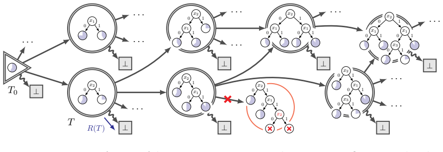
Generative Flow Networks (GFlowNets) are a class of probabilistic models that sample discrete, compositional objects by treating generation as a sequence of decisions. The thesis establishes that if a flow on a directed acyclic graph satisfies the flow matching condition — the sum of incoming edge flows equals the sum of outgoing edge flows at every non-initial state — and if the flow through each terminating edge is set to the target weight $R(x)$, then the induced forward policy samples $x$ with probability proportional to $R(x)$. This turns the problem of sampling from an intractable distribution, such as a Bayesian posterior over DAGs, into a scalable optimization problem over edge flows. The second half of the thesis applies this idea to Bayesian structure learning, approximating posteriors over Bayesian network structures and their parameters from observational and experimental data.

What carries the argument

The load-bearing object is a Markovian flow network on a pointed DAG: a non-negative edge flow $F(s\to s')$ with a single source $s_0$ and a single sink $\bot$. The flow matching condition enforces conservation at every non-initial state; the boundary condition $F(x\to\bot)=R(x)$ fixes the terminating flows. The identity that carries the argument is the induced forward policy $P_F^\star(s'|s)=F(s\to s')/F(s)$, which, by Proposition 3.1.8, samples terminating states exactly with probability $F(x\to\bot)/Z^\star$. Detailed balance, trajectory balance, and sub-trajectory balance are alternative re-expressions of the same conservation law at transition, full-trajectory, and partial-trajectory granularity, each usable as a training loss.

What would settle it

On a small, fully enumerable state space (for example, all DAGs on four nodes), compute the exact terminating-state distribution $P_F^\top(x)$ by dynamic programming, train a GFlowNet with a flow matching loss, and test whether the learned distribution approaches $R(x)/Z$ as training time and capacity grow; a persistent gap would falsify the claim that flow matching suffices for sampling.

Watch

Extended reading notes

Core claim

The central claim is that a non-negative reward function $R$ on a finite set of compositional objects can be realized as the terminating flow of a Markovian flow network. Setting $F(x\to\bot)=R(x)$ on each terminating edge and choosing edge flows satisfying the flow matching condition $\sum_{s\in\mathrm{Pa}(s')}F(s\to s')=\sum_{s''\in\mathrm{Ch}(s')}F(s'\to s'')$ at every non-initial state yields a forward policy $P_F(s'|s)=F(s\to s')/F(s)$ whose terminating-state distribution is exactly $R(x)/\sum_x R(x)$ (Proposition 3.1.8). The thesis further claims that this conservation law can be turned into a family of learning objectives — flow matching, detailed balance, trajectory balance, and sub-trajectory balance — and that training a neural-network policy against these losses yields an amortized sampler that approximates the target distribution, with convergence guarantees for exact flows. In structure learning, this yields DAG-GFlowNet for the marginal posterior over graphs and JSP-GFN for the joint posterior over graph and parameters, and the Markov-chain view extends the construction to continuous state spaces.

Load-bearing premise

The practical claim assumes that a parametric flow trained with flow-matching losses can be driven close enough to exact conservation over a huge discrete space; the theorems are exact only for exactly consistent flows and do not bound the error from finite-sample, function-approximation training.

Editorial extensions

If this is right

  • A GFlowNet trained with a flow matching loss can sample DAGs from the Bayesian posterior $P(G|D)$ rather than from a path-count-biased distribution, because the conservation law cancels trajectory multiplicities.
  • Off-policy training with a behavior policy can be used to improve exploration without changing the target distribution, and the convergence guarantees hold for the exact flow matching objectives.
  • GFlowNets and maximum-entropy reinforcement learning are equivalent after a reward correction, so the known multi-path bias of MaxEnt RL disappears when the reward is corrected as in Chapter 5.
  • The Markov-chain perspective extends GFlowNets to continuous and general state spaces, giving generalized detailed balance and trajectory balance conditions.
  • A single GFlowNet can approximate the joint posterior over the structure and the parameters of a Bayesian network, with DAG-GFlowNet as a special case.

Reading between the lines

Editorial extensions of the paper, not claims the author makes directly.

  • A reader could test the practical limit directly: on small enumerable state spaces, compute $P_F^\top(x)$ exactly by dynamic programming and measure how the flow-matching residual shrinks with capacity; this would separate training error from representational bias.
  • The same conservation-law sampler suggests an amortized proposal for MCMC or a reusable sampler for other discrete combinatorial objects, a connection the thesis only touches on.
  • Because the exact theorems are for exact flows, the practical quality of a GFlowNet may be predicted by the degree to which learned edge flows satisfy conservation at intermediate states; monitoring this residual is an implicit diagnostic.
Share X Bluesky LinkedIn Reddit HN

Signed reviews

No signed human review yet.

Editorial analysis

A structured set of objections, weighed in public.

Desk editor's note, referee report, and a circularity audit.

Referee Report

3 major / 4 minor

Summary. The thesis develops the theory of Generative Flow Networks (GFlowNets) as a class of sequential, amortized generative models for sampling from unnormalized distributions over discrete and compositional objects, and applies them to Bayesian structure learning. Part I introduces flow networks, defines Markovian flows, and proves that exact flows satisfying the flow matching condition (3.2.1), detailed balance (3.2.21), trajectory balance (3.2.31), or sub-trajectory balance (3.2.49) conditions are equivalent characterizations of a unique Markovian flow; Proposition 3.1.8 shows that the terminating distribution of such a flow is the normalized terminating edge flow. The thesis also connects GFlowNets to maximum entropy reinforcement learning and variational inference, and extends them to general state spaces. Part II constructs GFlowNets over DAGs, approximates the Bayesian posterior over structures (DAG-GFlowNet) and over structures and parameters jointly (JSP-GFN), and validates the approximations against exact posteriors computed by dynamic programming on small graphs and against MCMC baselines.

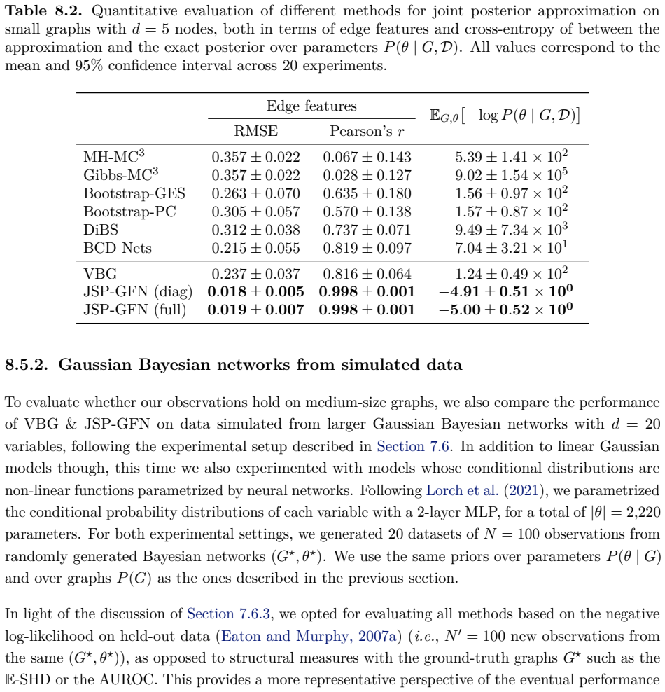
Significance. If the central claims hold, GFlowNets offer a principled and scalable alternative to MCMC for posterior inference over discrete structures, with clear connections to variational inference and max-entropy RL. The manuscript's strengths include the careful proofs of the flow conditions, the explicit empirical check against exact posterior enumeration for small graphs (Section 7.5), the integration of interventional and observational data (Section 7.7), and the candid limitation sections (7.4.3, 7.4.4, 8.3.5). The main caveat is that the exact-flow theory does not by itself justify the trained parametric approximation; the degree to which this gap is quantified or appropriately labeled determines whether the application claims are fully supported.

major comments (3)
  1. [§4.2.1; Prop. 3.1.8; Thm. 3.2.1] The central practical claim is that a trained GFlowNet samples approximately from the target reward distribution. Proposition 3.1.8 and Theorem 3.2.1 establish this only for exact Markovian flows satisfying the flow matching condition (3.2.1) and the boundary reward F(x→⊥)=R(x). The training losses in Section 4.2.1 minimize sampled residuals; their global optimum is zero at best on the support of the training distribution, and nothing in the presentation ensures that the parametric family contains a valid flow or that the training distribution covers the state space. The limitation sections 7.4.3, 7.4.4, and 8.3.5 acknowledge this gap, but provide no quantitative bound. Please either supply an error bound (for example, total variation distance in terms of the expected flow-matching residual and a coverage or exploration term) or explicitly reframe the practical claims as heuristic approximations.
  2. [§4.2.3] The chapter introduction promises 'novel convergence guarantees of the approximate distribution towards the target' and Section 4.2.3 is titled 'Convergence guarantees'. The precise assumptions of these guarantees should be stated clearly. If they require exact minimization of the flow-matching loss over a hypothesis class that contains a valid flow, or access to the full training distribution, then they do not cover the finite-capacity, finite-sample training used in Chapters 7 and 8, and the application chapters remain conditional on an unquantified approximation error.
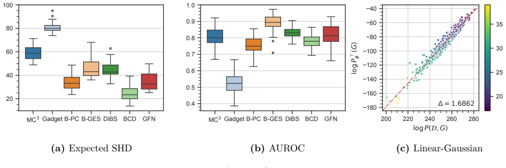
  3. [§7.5, §7.6.3] The exact-posterior comparison in Section 7.5 is limited to small graphs, while the medium-scale experiments (d=20) rely on metrics whose limitations are themselves acknowledged in Section 7.6.3. The thesis should either provide a quantitative calibration of those metrics (for example, by comparing expected SHD and AUROC against exact posteriors on graphs small enough for enumeration) or temper the scaling claims accordingly, so that the reader can distinguish validated accuracy from heuristic evaluation.
minor comments (4)
  1. [Résumé, p. iii] The French text reads 'lesréseaux à flots génératifs'; there is a missing space between 'les' and 'réseaux'.
  2. [Figure 2.2 caption] The caption uses 'quicunx'; the correct spelling is 'quincunx'.
  3. [Glossary, p. xiii] The glossary entry for 'P⊗T F' has inconsistent sub- and superscript rendering; please ensure it matches the notation used in Appendix A.
  4. [Conclusion] Since Sections 7.4.3, 7.4.4, and 8.3.5 each discuss limitations in different places, a consolidated limitations paragraph in the Conclusion that relates these caveats to the theoretical guarantees of Part I would help the reader assess the scope of the contributions.

Circularity Check

0 steps flagged · score 0.0 of 10

No circularity: the flow-matching theorem is proved in-text, the reward is an input, and the acknowledged approximation gap is a limitation, not a definitional reduction.

full rationale

Walking the derivation chain: the target distribution P*(x)=exp(-E(x))/Z is an input reward, not a quantity derived from the fitted model. Proposition 3.1.8 shows that a valid flow with terminating edge flow F(x->bottom)=R(x) induces the terminating distribution R(x)/Z; the proof uses Lemmas 3.1.6 and Proposition 3.1.4, not the target distribution. Theorem 3.2.1 proves that the flow matching condition (3.2.1) characterizes the edge flows of a unique Markovian flow, with a full proof in the text rather than an imported uniqueness claim. The training objectives in Section 4.2.1 minimize flow-matching residuals whose global zero is exactly the flow matching condition, and the convergence guarantees in Section 4.2.3 concern that exact minimization. The manuscript explicitly acknowledges in Sections 7.4.3, 7.4.4, and 8.3.5 that finite-sample, function-approximation, and training-distribution coverage gaps are not bounded; this is an honest limitation, not a circular step, because the theory is stated as a sufficiency result for exact flows. Empirical validation in Section 7.5.1 compares against exact posteriors computed by dynamic programming, an external benchmark, so the evaluation does not reuse GFlowNet outputs as ground truth. Although the thesis builds on several papers by the same author, the load-bearing theorems are restated and proved in the manuscript, so the self-citations are not load-bearing arguments. No fitted parameter is renamed as a prediction, no known result is merely relabeled, and no ansatz is smuggled in via citation. The derivation is self-contained relative to its stated assumptions.

Assumptions & free parameters 2 free parameters · 5 assumptions · 2 invented entities

The theoretical construction relies on standard graph/DAG assumptions and on the existence of a strictly positive flow satisfying conservation; the empirical structure-learning chapters additionally depend on faithfulness and on the chosen Bayesian scores as the target. No physical entities are posited; flows are mathematical bookkeeping with testable sampling consequences.

free parameters (2)
  • temperature alpha in MaxEnt RL equivalence = 1 (set by assumption)
    Section 2.3.1 states the entropy regularization temperature is assumed to be 1 for simplicity; changing it changes the target distribution to P proportional to exp(R/alpha).
  • prior hyperparameters for BDe/BGe scores = not specified in thesis
    In the structure learning experiments, the Bayesian score depends on user-chosen priors (e.g., equivalent sample size); these affect the posterior being approximated.
assumptions (5)
  • domain assumption Faithfulness: the data-generating distribution is faithful to the true DAG (Section 1.4.1).
    Used to justify structure identifiability up to Markov equivalence; assumed throughout the thesis without further mention.
  • standard math The state space is a finite pointed DAG with a unique source and sink (Definitions 2.2.1-2.2.3).
    All flow-matching theorems rely on this structure; extensions to cyclic/continuous spaces (Chapter 6) require additional Harris recurrence conditions.
  • ad hoc to paper Existence of a strictly positive Markovian flow matching the boundary reward (implicit in Theorem 3.2.1).
    The flow matching theorem requires edge flows with positive denominators at every state; in practice the learned parametric flow must keep all relevant flows nonzero.
  • domain assumption In Bayesian structure learning, the marginal likelihood (BGe/BDe score) is computable and used as the unnormalized posterior (Section 7.1, Appendix B).
    The target posterior is defined by this score; the method approximates it, but the score itself is assumed to be the correct target.
  • domain assumption For continuous-state extensions, the generalized Markov chain is Harris recurrent with an accessible atom (Section 6.2).
    Needed to guarantee convergence of the generalized GFlowNet process to the target measure.
invented entities (2)
  • Flow (trajectory flow, state flow, edge flow) independent evidence
    purpose: Auxiliary non-negative bookkeeping quantity over trajectories whose conservation yields the sampling policy; termination edge flows are set to the target reward.
    The flow's validity is testable through the induced sampling distribution against exact enumeration; however it is a mathematical construct, not an observed quantity.
  • Generative Flow Network (GFlowNet) as a model class independent evidence
    purpose: A family of sequential generative models trained to match a target distribution over compositional objects.
    Falsifiable via empirical comparisons to exact posteriors and MCMC on small graphs; no physical reality is claimed.

how reviews work

0 comments
Cite this review

Pith. "Pith review of Generative Flow Networks: Theory and Applications to Structure Learning." pith.science (2026). https://pith.science/paper/53XSQA62

@misc{pith2026250105498,
  author       = {Pith},
  title        = {Pith review of: Generative Flow Networks: Theory and Applications to Structure Learning},
  year         = {2026},
  howpublished = {\url{https://pith.science/paper/53XSQA62}},
  note         = {Machine review of arXiv:2501.05498}
}
read the original abstract

Without any assumptions about data generation, multiple causal models may explain our observations equally well. To avoid selecting a single arbitrary model that could result in unsafe decisions if it does not match reality, it is therefore essential to maintain a notion of epistemic uncertainty about our possible candidates. This thesis studies the problem of structure learning from a Bayesian perspective, approximating the posterior distribution over the structure of a causal model, represented as a directed acyclic graph (DAG), given data. It introduces Generative Flow Networks (GFlowNets), a novel class of probabilistic models designed for modeling distributions over discrete and compositional objects such as graphs. They treat generation as a sequential decision making problem, constructing samples of a target distribution defined up to a normalization constant piece by piece. In the first part of this thesis, we present the mathematical foundations of GFlowNets, their connections to existing domains of machine learning and statistics such as variational inference and reinforcement learning, and their extensions beyond discrete problems. In the second part of this thesis, we show how GFlowNets can approximate the posterior distribution over DAG structures of causal Bayesian Networks, along with the parameters of its causal mechanisms, given observational and experimental data.

Figures
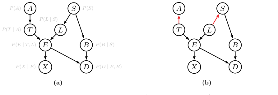
Figures reproduced from arXiv: 2501.05498 by the authors.

Figure 1.1
Figure 1.1. Factorization of the joint distribution P(A, B, D, E, L, S, T, X) as a Bayesian network (Lauritzen and Spiegelhalter, 1988). (a) Illustration of the structure of a Bayesian network, with the corresponding conditional distributions. (b) An example of a Markov equivalent Bayesian network representing the same conditional independencies, where the edges A → T & S → L have been reversed. the joint distribution factorize… view at source ↗
Figure 1
Figure 1. a [PITH_FULL_IMAGE:figures/full_fig_p024_1.png] view at source ↗
Figure 1
Figure 1. a [PITH_FULL_IMAGE:figures/full_fig_p025_1.png] view at source ↗
Figures from the paper (93 more)
Figure 1
Figure 1. Figure 1: a [PITH_FULL_IMAGE:figures/full_fig_p033_1.png]
Figure 1.2
Figure 1.2. Figure 1.2: Example of a distribution violating the faithfulness assumption. (a) Example of a Bayesian network with its conditional distributions in the decomposition of P(X, Y, Z). (b) The only conditional independence statements one can extract from P(X, Y, Z) are X ⊥⊥ Z & X ̸…
Figure 1
Figure 1. Figure 1 [PITH_FULL_IMAGE:figures/full_fig_p037_1.png]
Figure 1.3
Figure 1.3. Figure 1.3: The effect of an intervention on the causal graph. (a) Example of a causal graph representing a family of distributions, including the joint (observational) distribution P(A, B, D, E, L, S, T, X). (b) The mutilated graph corresponding to intervening on the random var…
Figure 2
Figure 2. Figure 2 [PITH_FULL_IMAGE:figures/full_fig_p043_2.png]
Figure 2.1
Figure 2.1. Figure 2.1: Examples of compositional objects. An organic molecule is a collection of molecular fragments assembled together. A protein sequence is a sequence of amino acids. An inorganic material is composed multiple elements (often organized as a crystal; Mila AI4Science et al…
Figure 2
Figure 2. Figure 2: a [PITH_FULL_IMAGE:figures/full_fig_p044_2.png]
Figure 2.2
Figure 2.2. Figure 2.2: The Galton board. (a) Visualization of the Galton board, where blue beads fall down the apparatus into one of the five bins. (b) A bead falling into a specific bin may take multiple paths, bouncing off a different sequence of pins. (c) Representation of the Galton bo…
Figure 2
Figure 2. Figure 2: b [PITH_FULL_IMAGE:figures/full_fig_p045_2.png]
Figure 2
Figure 2. Figure 2: c [PITH_FULL_IMAGE:figures/full_fig_p046_2.png]
Figure 3
Figure 3. Figure 3 [PITH_FULL_IMAGE:figures/full_fig_p046_3.png]
Figure 2
Figure 2. Figure 2: c [PITH_FULL_IMAGE:figures/full_fig_p047_2.png]
Figure 3
Figure 3. Figure 3 [PITH_FULL_IMAGE:figures/full_fig_p049_3.png]
Figure 2
Figure 2. Figure 2 [PITH_FULL_IMAGE:figures/full_fig_p049_2.png]
Figure 2
Figure 2. Figure 2 [PITH_FULL_IMAGE:figures/full_fig_p050_2.png]
Figure 2.3
Figure 2.3. Figure 2.3: Pointed DAG for the generation of small organic molecules. At each step of generation, a new molecular fragment chosen from a fixed vocabulary of fragments is added at some end of the partial molecule. The process eventually leads to fully formed molecules (e.g., asp…
Figure 2
Figure 2. Figure 2 [PITH_FULL_IMAGE:figures/full_fig_p051_2.png]
Figure 2.4
Figure 2.4. Figure 2.4: Autoregressive sampling from a discrete factor graph, viewed from the perspective of sequential generation in a pointed DAG. (Left) An example of a factor graph over 3 binary random variables X1, X2, and X3, with 3 factors ψ1, ψ2, and ψ3. The energy function associat…
Figure 2
Figure 2. Figure 2 [PITH_FULL_IMAGE:figures/full_fig_p052_2.png]
Figure 2
Figure 2. Figure 2 [PITH_FULL_IMAGE:figures/full_fig_p055_2.png]
Figure 2.5
Figure 2.5. Figure 2.5: Illustration of the bias of the terminating state distribution associated with π ⋆ MaxEnt on a soft MDP with a DAG structure. The labels on each transition of the MDP corresponds to the reward function, satisfying (2.3.1) (i.e., sparse reward setting). The terminatin…
Figure 2
Figure 2. Figure 2 [PITH_FULL_IMAGE:figures/full_fig_p056_2.png]
Figure 3.1
Figure 3.1. Figure 3.1: Illustration of a flow network. (a) A flow of particles traverses the network of pipes, from s0 to the terminal state ⊥ (illustrated by the gradual change in color). The edge flow F ⋆ (s → s ′ ) quantifies the “amount of particles” going through s → s ′ . (b) Represe…
Figure 3
Figure 3. Figure 3: a [PITH_FULL_IMAGE:figures/full_fig_p060_3.png]
Figure 3
Figure 3. Figure 3 [PITH_FULL_IMAGE:figures/full_fig_p064_3.png]
Figure 3.2
Figure 3.2. Figure 3.2: Examples of Markovian, non-Markovian, and equivalent flows. The flows F ⋆ 2 & F ⋆ 4 are Markovian, whereas F ⋆ 1 & F ⋆ 3 are not. The first two flows are equivalent F ⋆ 1 ∼ F ⋆ 2 . Similarly, F ⋆ 3 ∼ F ⋆ 4 , but they are not equivalent to F ⋆ 1 and F ⋆ 2 . All these …
Figure 3
Figure 3. Figure 3 [PITH_FULL_IMAGE:figures/full_fig_p068_3.png]
Figure 3
Figure 3. Figure 3 [PITH_FULL_IMAGE:figures/full_fig_p069_3.png]
Figure 3.3
Figure 3.3. Figure 3.3: Illustration of the flow matching conditions. (a) The flow matching condition operates at the level of states s ′ (Section 3.2.1) (b) The detailed balance condition operates at the level of transitions (Section 3.2.2). (c) The trajectory balance condition operates at…
Figure 3.4
Figure 3.4. Figure 3.4: Decomposition of a complete trajectory going through the transition s → s ′ into a prefix ←−τ to a parent s¯, a transition s¯ → s, the transition s → s ′ , and a suffix −→τ . from s0 to some parent s¯ ∈ PaG(s), (2) a transition s¯ → s, (3) the transition s → s ′ , an…
Figure 3.5
Figure 3.5. Figure 3.5: Analogy between the flow matching condition and Kirchhoff’s current law. (a) A Markovian flow network with the edge flow defined at each transition. (b) An equivalent electrical circuit with a power source and 6 resistors. The values of the resistances are chosen in …
Figure 3
Figure 3. Figure 3 [PITH_FULL_IMAGE:figures/full_fig_p073_3.png]
Figure 3
Figure 3. Figure 3: a [PITH_FULL_IMAGE:figures/full_fig_p074_3.png]
Figure 3.6
Figure 3.6. Figure 3.6: Counter-example of the sufficiency of the sub-trajectory balance condition. We consider all the partial trajectories of length 2 in the pointed DAG (left), and write the corresponding sub￾trajectory balance condition for each trajectory (right; simplified). This syst…
Figure 3
Figure 3. Figure 3 [PITH_FULL_IMAGE:figures/full_fig_p080_3.png]
Figure 3
Figure 3. Figure 3: e [PITH_FULL_IMAGE:figures/full_fig_p081_3.png]
Figure 3
Figure 3. Figure 3 [PITH_FULL_IMAGE:figures/full_fig_p082_3.png]
Figure 3.7
Figure 3.7. Figure 3.7: Example of a state-conditional flow network. (a) The original Markovian flow F ⋆ , with the edge flows indicated at each transition. (b) The subgraph of states reachable from s2; there is a flow through (s0, s1, s5, ⊥) that contributes to F ⋆ (s5 → ⊥), but is not acc…
Figure 3
Figure 3. Figure 3: b [PITH_FULL_IMAGE:figures/full_fig_p084_3.png]
Figure 2
Figure 2. Figure 2 [PITH_FULL_IMAGE:figures/full_fig_p085_2.png]
Figure 4.1
Figure 4.1. Figure 4.1: Difference between a flow network and a generative flow network. (a) A flow network has a flow which is completely unrestricted, which only needs to satisfy some flow matching conditions. (b) A generative flow network (GFlowNet) is a flow network satisfying some boun…
Figure 4
Figure 4. Figure 4 [PITH_FULL_IMAGE:figures/full_fig_p093_4.png]
Figure 4.2
Figure 4.2. Figure 4.2: Bayesian inference of decision tree structures with a generative flow network. This is an illustration of the pointed DAG G, each state being the structure of a decision tree. The shading at the leaves indicates the label proportions. A transition T → T ′ corresponds…
Figure 5
Figure 5. Figure 5 [PITH_FULL_IMAGE:figures/full_fig_p114_5.png]
Figure 5.1
Figure 5.1. Figure 5.1: Equivalence between objectives in MaxEnt RL, with corrected rewards, and the objectives in GFlowNets. The objectives are classified based on whether they operate at the level of (complete) trajectories (left), transitions (middle), or if all the states are terminatin…
Figure 5
Figure 5. Figure 5 [PITH_FULL_IMAGE:figures/full_fig_p120_5.png]
Figure 5.2
Figure 5.2. Figure 5.2: Revisiting sampling in a discrete factor graph of Section 2.2.5, with intermediate rewards. Instead of computing the energy of the whole terminating state E(x1, x2, x3) upon termination, there are some intermediate rewards along the way as soon as all the information…
Figure 5.3
Figure 5.3. Figure 5.3: Summary of the equivalences between the residuals in MaxEnt RL (top, in each box) and GFlowNet (bottom, in each box) objectives, using the classification of [PITH_FULL_IMAGE:figures/full_fig_p125_5_3.png]
Figure 6.1
Figure 6.1. Figure 6.1: Discrete GFlowNet as a recurrent Markov chain. (a) The pointed DAG structure of a GFlowNet, with the flow going from the initial state s0 to the terminal state ⊥. (b) The “wrapped-around” version of the same GFlowNet, where the initial state has been merged with the …
Figure 6
Figure 6. Figure 6 [PITH_FULL_IMAGE:figures/full_fig_p131_6.png]
Figure 6
Figure 6. Figure 6 [PITH_FULL_IMAGE:figures/full_fig_p134_6.png]
Figure 6.2
Figure 6.2. Figure 6.2: Construction of an atom via the splitting technique. (a) Illustration of the atom S0 = X × {1} created from X . Once the Markov chain reaches the atom S0, it transitions to its next state with the kernel ν(cot), independent of x. (b) The split chain Zn = (Xn, Yn), wh…
Figure 6
Figure 6. Figure 6 [PITH_FULL_IMAGE:figures/full_fig_p140_6.png]
Figure 6
Figure 6. Figure 6: b [PITH_FULL_IMAGE:figures/full_fig_p143_6.png]
Figure 6.3
Figure 6.3. Figure 6.3: Relation between the atom S0 for the split chain Zn = (Xn, Yn) and the set S1. The value ∗ indicates that the value can be arbitrary. Returning to S0 at random time σS0 happens exactly one step before hitting the set S1 (corresponding to hitting the terminating state…
Figure 6
Figure 6. Figure 6 [PITH_FULL_IMAGE:figures/full_fig_p152_6.png]
Figure 2
Figure 2. Figure 2 [PITH_FULL_IMAGE:figures/full_fig_p159_2.png]
Figure 7
Figure 7. Figure 7 [PITH_FULL_IMAGE:figures/full_fig_p161_7.png]
Figure 7.1
Figure 7.1. Figure 7.1: Illustration of the moves made by a proposal distribution in structure Markov chain Monte Carlo, where starting from a certain DAG, we can either add, subtract (Madigan and York, 1995), or reverse (Grzegorczyk and Husmeier, 2008) a single edge. 7.1.2. Variational inf…
Figure 7.2
Figure 7.2. Figure 7.2: Structure of a GFlowNet over DAGs. The states of the GFlowNet correspond to DAGs, with the initial state G0 being the completely disconnected graph. Each state G is terminating (i.e., connected to the terminal state ⊥, represented by blue arrows for brevity) and asso…
Figure 7
Figure 7. Figure 7 [PITH_FULL_IMAGE:figures/full_fig_p164_7.png]
Figure 7
Figure 7. Figure 7 [PITH_FULL_IMAGE:figures/full_fig_p166_7.png]
Figure 7.3
Figure 7.3. Figure 7.3: Online update of the mask M. The mask Mt associated with Gt represents (in black) the edges that can be added to Gt to obtain a valid DAG. Mt is decomposed in two parts (Proposition 7.2.2): (1) the adjacency matrix of Gt (top) and (2) the transpose of its transitive …
Figure 7
Figure 7. Figure 7 [PITH_FULL_IMAGE:figures/full_fig_p174_7.png]
Figure 7.4
Figure 7.4. Figure 7.4: Linear Transformer architecture for the forward transition probabilities Pϕ(· | G). The input graph G is encoded as a set of d 2 possible edges (including self-loops); each directed edge is embedded using the embeddings of its source and target, with an additional ve…
Figure 7
Figure 7. Figure 7 [PITH_FULL_IMAGE:figures/full_fig_p181_7.png]
Figure 7.5
Figure 7.5. Figure 7.5: Comparison between the exact posterior distribution and the approximation from DAG-GFlowNet, for different structural features: (a) edge features Xi → Xj , (b) path features Xi ⇝ Xj , and (c) Markov blanket features Xi ∼M Xj . Each point corresponds to a feature (i.e…
Figure 7
Figure 7. Figure 7: a [PITH_FULL_IMAGE:figures/full_fig_p183_7.png]
Figure 7.6
Figure 7.6. Figure 7.6: Comparison of the edge features computed either with GFlowNet objectives, or the Reverse KL objective in (4.3.28). Performance is reported as the root mean square error (RMSE) between the edge features computed with the exact posterior P(G | D) and the approximation …
Figure 7.7
Figure 7.7. Figure 7.7: Bayesian structure learning of linear-Gaussian Bayesian networks with d = 20 nodes. Results for (a) E-SHD (lower is better) & (b) AUROC (higher is better) are aggregated over 25 randomly generated datasets D. Labels: B-PC = Bootstrap-PC, B-GES = Bootstrap-GES, BCD = …
Figure 7
Figure 7. Figure 7: c [PITH_FULL_IMAGE:figures/full_fig_p186_7.png]
Figure 7
Figure 7. Figure 7: a [PITH_FULL_IMAGE:figures/full_fig_p187_7.png]
Figure 8
Figure 8. Figure 8 [PITH_FULL_IMAGE:figures/full_fig_p187_8.png]
Figure 7
Figure 7. Figure 7 [PITH_FULL_IMAGE:figures/full_fig_p188_7.png]
Figure 7.8
Figure 7.8. Figure 7.8: Coverage of the posterior approximations learned on flow cytometry data. Each point corresponds to a sampled Markov equivalence class, and its size represents the number of unique DAGs sampled from the posterior approximation (with 1,000 samples) in the MEC. The x-ax…
Figure 7
Figure 7. Figure 7 [PITH_FULL_IMAGE:figures/full_fig_p189_7.png]
Figure 7.9
Figure 7.9. Figure 7.9: Exhaustive structure of a GFlowNet over DAGs with d = 3 nodes. This pointed DAG contains 25 states (one for each possible DAG) and 48 edges. The initial state is the empty graph at the center of the figure. 172 [PITH_FULL_IMAGE:figures/full_fig_p191_7_9.png]
Figure 8
Figure 8. Figure 8 [PITH_FULL_IMAGE:figures/full_fig_p200_8.png]
Figure 8.1
Figure 8.1. Figure 8.1: Structure of JSP-GFN to approximate the joint posterior distribution P(G, θ | D). A graph G and the parameters θ are constructed as follows: starting from the empty graph G0, (1) the graph G is first generated one edge at a time (blue), as in (Deleu et al., 2022a). T…
Figure 8
Figure 8. Figure 8 [PITH_FULL_IMAGE:figures/full_fig_p202_8.png]
Figure 8.2
Figure 8.2. Figure 8.2: Sub-trajectory balance conditions for undirected paths of length 3 (red) & 2 (blue) considered here, with an illustration of these paths on an excerpt of the pointed DAG of [PITH_FULL_IMAGE:figures/full_fig_p207_8_2.png]
Figure 8
Figure 8. Figure 8: b [PITH_FULL_IMAGE:figures/full_fig_p209_8.png]
Figure 8.3
Figure 8.3. Figure 8.3: Conditional dependencies between the DAG G, the parameters θ, and datapoints x & x ′ ∈ D. (a) The conditional dependencies represented as a (higher level) Bayesian network. (b) The effect of conditioning only on G; this leaves an open path between x and x ′ through θ…
Figure 8
Figure 8. Figure 8 [PITH_FULL_IMAGE:figures/full_fig_p212_8.png]
Figure 7
Figure 7. Figure 7 [PITH_FULL_IMAGE:figures/full_fig_p212_7.png]
Figure 8.4
Figure 8.4. Figure 8.4: Comparison between the exact posterior distribution and the approximation from JSP-GFN, for different structural features. (a-c) the posterior approximation over parameters P(θ | G,stop) is parametrized as a Normal distribution with diagonal covariance (JSP-GFN (diag…
Figure 8
Figure 8. Figure 8: a [PITH_FULL_IMAGE:figures/full_fig_p214_8.png]
Figure 7
Figure 7. Figure 7: c [PITH_FULL_IMAGE:figures/full_fig_p214_7.png]
Figure 8.5
Figure 8.5. Figure 8.5: Evaluation of JSP-GFN on Gaussian Bayesian networks with d = 20 variables. (a￾b) Comparison of the negative log-likelihood on N′ = 100 held-out observations for different Bayesian structure learning methods, aggregated across 20 experiments on different datasets D. (…
Figure 8
Figure 8. Figure 8: c [PITH_FULL_IMAGE:figures/full_fig_p215_8.png]
Figure 8.6
Figure 8.6. Figure 8.6: Performance of JSP-GFN on the inference of protein signaling networks with flow cytometry data (Sachs et al., 2005). (a) Linear correlation between the log-reward (x-axis) and terminating state log-probability (y-axis) on a model trained with a subsampled dataset. Ea…
Figure 8
Figure 8. Figure 8: c [PITH_FULL_IMAGE:figures/full_fig_p216_8.png]
Figure 8
Figure 8. Figure 8: c [PITH_FULL_IMAGE:figures/full_fig_p218_8.png]

Discussion (0). Continue with ORCID to comment.

Forward citations

Cited by 2 Pith papers

Reviewed papers in the Pith corpus that reference this work. Sorted by Pith novelty score. Full citation record

  1. Revisiting Non-Acyclic GFlowNets in Discrete Environments

    cs.LG 2025-02 accept novelty 7.0 of 10

    In cyclic discrete environments, GFlowNet flows are expected visit counts, and training a non-acyclic GFlowNet with the smallest expected trajectory length is equivalent to minimizing total flow.

  2. Efficient Diversity-Preserving Diffusion Alignment via Gradient-Informed GFlowNets

    cs.LG 2024-12 conditional novelty 7.0 of 10

    A gradient-informed GFlowNet objective, residual nabla-DB, finetunes diffusion models to sample according to a reward while preserving diversity and prior knowledge.

Reference graph

Works this paper leans on

3 extracted references · 3 canonical work pages · cited by 2 Pith papers

  1. [1]

    wake-sleep

    Raj Agrawal, Chandler Squires, Karren Yang, Karthikeyan Shanmugam, and Caroline Uhler (2019). ABCD-Strategy: Budgeted Experimental Design for Targeted Causal Structure Discovery. International Conference on Artificial Intelligence and Statistics (AISTATS)(cited on pp. 193, 200). Hirotugu Akaike (1974). A New Look at the Statistical Model Identification.IE...

  2. [3]

    This concludes the proof, showing that invariance also holds ats0

    Therefore ∑ s∈S F (s)PF (s0|s) = ∑ s∈S ∞∑ n=0 F (s0)Es0 [ 1(n<σ s0)1(Xn =s) ] PF (s0|s) (A.2.5) =F (s0) ∑ s∈S ∞∑ n=1 Es0 [ 1(σs0 =n)1(Xn−1 =s) ] (A.2.6) =F (s0) ∞∑ n=1 Es0 [ 1(σs0 =n) ∑ s∈S 1(Xn−1 =s) /bracehtipupleft/bracehtipdownright/bracehtipdownleft/bracehtipupright = 1 ] (A.2.7) =F (s0) ∞∑ n=1 Es0 [ 1(σs0 =n) ] =F (s0), (A.2.8) where we substitutedF...

  3. [2019]

    Proposition A.1.2 (Data processing inequality)

    and recalled for completeness, plays an important role in proving Proposition 4.3.1, which establishes a bound on thef-divergence between the terminating state probability distribution of a GFlowNet and the target Gibbs distribution, in terms of the f-divergence between distributions over complete trajectories (Malkin et al., 2022). Proposition A.1.2 (Dat...

Pith tools

Reviewed August 10, 2026 · model on record in the stance chip above.