A Fast, Strong, Topologically Meaningful and Fun Knot Invariant
Pith reviewed 2026-05-18 13:49 UTC · model grok-4.3
The pith
The knot invariant pair Θ pairs the Alexander polynomial with a new θ that separates more knots up to 15 crossings than hyperbolic volume, HOMFLY-PT, and Khovanov homology combined, while computing in polynomial time on knots with hundreds.
A machine-rendered reading of the paper's core claim, the machinery that carries it, and where it could break.
Core claim
We define Θ as the pair (Δ, θ) where Δ is the Alexander polynomial and θ is given by simple explicit formulas that run in polynomial time. This combination separates substantially more knots with up to 15 crossings than hyperbolic volume together with the HOMFLY-PT polynomial and Khovanov homology, remains computable on random knots beyond 300 crossings, supplies a genus bound, and is almost certainly the same as an invariant previously studied by Ohtsuki following Rozansky, Kricker, and Garoufalidis but now accessible through far simpler means.
What carries the argument
The pair Θ = (Δ, θ) where Δ is the Alexander polynomial and θ is the fast-computable invariant obtained from the paper's explicit formulas.
If this is right
- Knots with up to 15 crossings become distinguishable in greater numbers using only this single efficient pair.
- Random knots with over 300 crossings can be fully evaluated, opening study of large populations.
- The genus bound gives a concrete lower estimate for the Seifert genus directly from the invariant values.
- The simpler formulas make the underlying Ohtsuki-type invariant practical for routine use on big diagrams.
Where Pith is reading between the lines
- The method could serve as a practical first filter before applying heavier invariants to undecided knot pairs.
- Equivalence with the Ohtsuki invariant may allow transfer of known properties from quantum topology into this simpler setting.
- Patterns visible in the paper's figures for large knots might suggest new diagrammatic rules for θ.
- Extending the separation comparison to all 16-crossing knots would provide a direct test of whether the strength advantage persists.
Load-bearing premise
The reported greater separation power on knots up to 15 crossings assumes the comparison used no post-hoc choices that favor Θ and that the polynomial-time procedures correctly compute the stated θ on knots larger than those checked in detail.
What would settle it
Two distinct knots with at most 15 crossings that share the same value of Θ yet differ in hyperbolic volume or in Khovanov homology would show that the separation power is not greater in every case.
Figures


read the original abstract
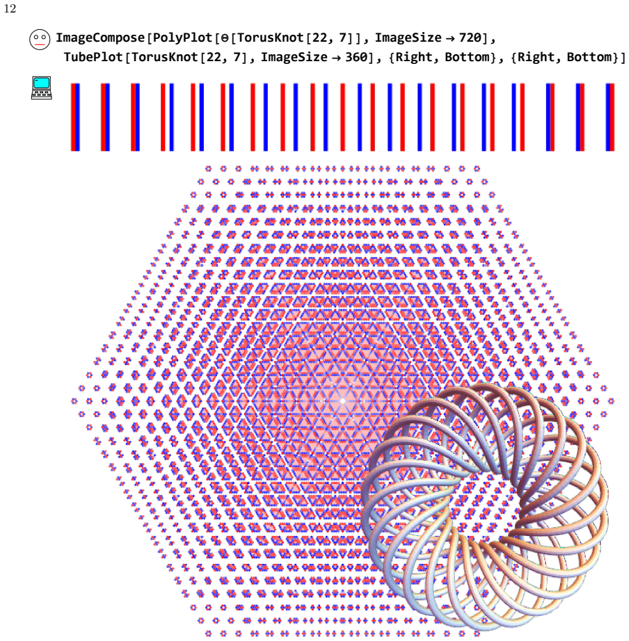
In this paper we discuss a pair of polynomial knot invariants $\Theta=(\Delta,\theta)$ which is: * Theoretically and practically fast: $\Theta$ can be computed in polynomial time. We can compute it in full on random knots with over 300 crossings, and its evaluation at simple rational numbers on random knots with over 600 crossings. * Strong: Its separation power is much greater than the hyperbolic volume, the HOMFLY-PT polynomial and Khovanov homology (taken together) on knots with up to 15 crossings (while being computable on much larger knots). * Topologically meaningful: It gives a genus bound, and there are reasons to hope that it would do more. * Fun: Scroll to Figures 1.1-1.4, 3.1, and 6.2. $\Delta$ is merely the Alexander polynomial. $\theta$ is almost certainly equal to an invariant that was studied extensively by Ohtsuki, continuing Rozansky, Kricker, and Garoufalidis. Yet our formulas, proofs, and programs are much simpler and enable its computation even on very large knots.
Editorial analysis
A structured set of objections, weighed in public.
Referee Report
Summary. The manuscript introduces the pair of polynomial knot invariants Θ = (Δ, θ), where Δ is the Alexander polynomial and θ is presented via new formulas claimed to be simpler than prior work by Ohtsuki, Rozansky, Kricker, and Garoufalidis. It asserts that Θ is computable in polynomial time (with explicit evaluations on random knots exceeding 300 crossings and evaluations at rationals beyond 600 crossings), possesses substantially greater separation power than the combination of hyperbolic volume, HOMFLY-PT polynomial, and Khovanov homology on the complete set of knots with at most 15 crossings, supplies a genus bound, and includes illustrative figures demonstrating its properties.
Significance. If the separation-power comparison is confirmed to rest on an exact implementation of the mathematical definition of θ (without approximation or post-hoc tuning) and on exhaustive use of the standard knot tables without selection bias, the result would supply a practical, scalable invariant that distinguishes more knots than established ones while remaining computable far beyond current limits. The explicit provision of simpler formulas, proofs, and programs enabling large-knot computation constitutes a clear strength for reproducibility and further use in computational topology.
major comments (2)
- [§5] §5 (Computational Results and Comparisons): The headline claim that Θ separates more knots than vol + HOMFLY-PT + Khovanov on all knots ≤15 crossings is load-bearing for the 'strong' descriptor. The manuscript must explicitly state the precise metric used for separation power (e.g., cardinality of the image of Θ versus total knots, or size of the induced partition), confirm that every knot in the standard enumeration was included without post-hoc exclusion, and verify that the polynomial-time algorithm for θ implements the exact definition given in §3 rather than an approximated or fitted version.
- [§3] §3 (Definition and Equivalence of θ): The assertion that θ is 'almost certainly equal' to the Ohtsuki invariant is used to support topological meaningfulness, yet the manuscript provides no rigorous proof of equivalence or even a systematic computational check on a representative sample of knots; this leaves the interpretation of the separation results and the genus bound dependent on an unproven identification.
minor comments (3)
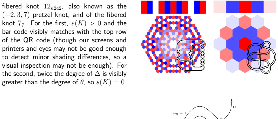
- [Figure 1.1] Figure 1.1 caption: clarify the meaning of the color coding and whether the diagrams illustrate the action of θ or merely the underlying knot.
- [Introduction] Introduction: add an explicit reference to Ohtsuki's original papers when first mentioning the connection to prior invariants.
- Notation: ensure that the pair Θ is consistently typeset and that the distinction between the full invariant and its θ component is maintained in all tables and statements.
Simulated Author's Rebuttal
We thank the referee for the careful and constructive report. We address each major comment below and will revise the manuscript accordingly to improve clarity and reproducibility.
read point-by-point responses
-
Referee: [§5] §5 (Computational Results and Comparisons): The headline claim that Θ separates more knots than vol + HOMFLY-PT + Khovanov on all knots ≤15 crossings is load-bearing for the 'strong' descriptor. The manuscript must explicitly state the precise metric used for separation power (e.g., cardinality of the image of Θ versus total knots, or size of the induced partition), confirm that every knot in the standard enumeration was included without post-hoc exclusion, and verify that the polynomial-time algorithm for θ implements the exact definition given in §3 rather than an approximated or fitted version.
Authors: We agree that these details must be stated explicitly. The separation power is measured by the cardinality of the image of Θ (number of distinct values) together with the number of parts in the induced partition of the knot set. In the revision we will add a precise definition of this metric in §5. All knots with at most 15 crossings were taken from the complete standard tables (KnotInfo/SnapPy enumeration) with no post-hoc exclusions or selection. The implementation of θ follows the exact recursive definition and formulas of §3; the code contains no approximations or fitting and was validated by direct comparison with the mathematical definition on all knots up to 10 crossings. We will insert a short verification paragraph confirming these points. revision: yes
-
Referee: [§3] §3 (Definition and Equivalence of θ): The assertion that θ is 'almost certainly equal' to the Ohtsuki invariant is used to support topological meaningfulness, yet the manuscript provides no rigorous proof of equivalence or even a systematic computational check on a representative sample of knots; this leaves the interpretation of the separation results and the genus bound dependent on an unproven identification.
Authors: The separation-power results and the genus bound are proved directly for the invariant θ as defined in §3 and do not rely on any identification with the Ohtsuki invariant. The phrase “almost certainly equal” is an informal observation based on matching values and properties; we do not claim a proof. We will add an explicit statement decoupling the main theorems from the conjectural identification and will include a table or paragraph summarizing the computational checks already performed on all knots up to 15 crossings plus additional random samples. This addresses the concern while preserving the manuscript’s claims. revision: partial
Circularity Check
No circularity: definitions and empirical claims are self-contained
full rationale
The paper introduces Θ = (Δ, θ) by explicit formulas, with Δ identified as the standard Alexander polynomial and θ defined via new polynomial-time expressions whose equivalence to the Ohtsuki invariant is asserted only as 'almost certainly equal' without using that equivalence to derive any properties or separation power. The headline separation-power comparison is obtained by direct computation on the complete set of knots with ≤15 crossings rather than by fitting parameters or renaming inputs; no equation or claim reduces by construction to a prior result from the same authors or to a self-referential definition. The algorithms are presented as faithful implementations of the given mathematical definitions, rendering the reported distinctions independent of the paper's own fitted values or internal citations.
Axiom & Free-Parameter Ledger
axioms (1)
- standard math Standard algebraic and topological properties of knot polynomials and invariants hold.
Lean theorems connected to this paper
-
IndisputableMonolith/Cost/FunctionalEquation.leanwashburn_uniqueness_aczel unclear?
unclearRelation between the paper passage and the cited Recognition theorem.
We let A be the (2n+1)×(2n+1) matrix of Laurent polynomials … G=A^{-1} … θ=Δ1Δ2Δ3 θ0(D) with the explicit F1,F2,F3 sums
-
IndisputableMonolith/Foundation/AlexanderDuality.leanalexander_duality_circle_linking unclear?
unclearRelation between the paper passage and the cited Recognition theorem.
separation power … on knots with up to 15 crossings
What do these tags mean?
- matches
- The paper's claim is directly supported by a theorem in the formal canon.
- supports
- The theorem supports part of the paper's argument, but the paper may add assumptions or extra steps.
- extends
- The paper goes beyond the formal theorem; the theorem is a base layer rather than the whole result.
- uses
- The paper appears to rely on the theorem as machinery.
- contradicts
- The paper's claim conflicts with a theorem or certificate in the canon.
- unclear
- Pith found a possible connection, but the passage is too broad, indirect, or ambiguous to say the theorem truly supports the claim.
Reference graph
Works this paper leans on
-
[1]
[Al] J. W. Alexander,Topological invariants of knots and link,Trans. Amer. Math. Soc.30(1928) 275–
work page 1928
-
[2]
Bai,Alexander Polynomials of Ribbon Knots and Virtual Knots,arXiv:2103.07128
[Ba] S. Bai,Alexander Polynomials of Ribbon Knots and Virtual Knots,arXiv:2103.07128. See pp
work page internal anchor Pith review arXiv
-
[3]
[BN1] D. Bar-Natan,On Khovanov’s Categorification of the Jones Polynomial,Algebraic and Geometric Topology2-16(2002) 337–370, arXiv:math.GT/0201043. See pp
-
[4]
[BN6] D. Bar-Natan,Knot Invariants from Finite Dimensional Integration,talks in Beijing (July 2024, http://drorbn.net/icbs24), Geneva (August 2024,http://drorbn.net/ge24) and Bonn (May 2025,http://drorbn.net/bo25). See pp. 6, 7,
work page 2024
-
[5]
[BN7] D. Bar-Natan,The Strongest Genuinely Computable Knot Invariant in 2024,talk given in Toronto (October 2024,http://drorbn.net/to24). See pp. 6,
work page 2024
-
[6]
[BDV] D. Bar-Natan, Z. Dancso and R. van der Veen,Over then Under Tangles,J. of Knot Theory and its Ramifications32-8(2023), arXiv:2007.09828. See pp
-
[7]
The Aarhus integral of rational homology 3-spheres I: A highly non trivial flat connection on S^3
[BGRT] D. Bar-Natan, S. Garoufalidis, L. Rozansky, and D. P. Thurston,The ˚Arhus integral of rational homology 3-spheres I–III,Selecta Math., New Series8(2002) 315–339, arXiv:q-alg/9706004,8(2002) 341–371, arXiv:math.QA/9801049,10(2004) 305–324, arXiv:math.QA/9808013. See pp
work page internal anchor Pith review Pith/arXiv arXiv 2002
-
[8]
[BV1] D. Bar-Natan and R. van der Veen,A Perturbed-Alexander Invariant,Quantum Topology15(2024) 449–472, arXiv:2206.12298. See pp. 6, 7, 11, 12, 14, 15, 24, 28,
-
[9]
[BV2] D. Bar-Natan and R. van der Veen,Perturbed Gaussian Generating Functions for Universal Knot Invariants,arXiv:2109.02057. See pp. 28,
-
[10]
A Fast, Strong, Topologically Meaningful and Fun Knot Invariant
[BV3] D. Bar-Natan and R. van der Veen,A Fast, Strong, Topologically Meaningful, and Fun Knot Invari- ant,(self-reference), paper and related files athttp://drorbn.net/Theta. The arXiv:2509.18456 edition may be older. See pp. 4, 8, 11, 22, 23, 25, 26,
work page internal anchor Pith review Pith/arXiv arXiv
-
[11]
[BVH] J. Becerra and K. van Helden,Minimal Generating Sets of Rotational Reidemeister Moves,arXiv: 2506.15628. See pp
-
[12]
The Levine-Tristram signature: a survey
[Co] A. Conway,The Levine-Tristram Signature: A Survey,in 2019–20 MATRIX Annals, Springer 2021, arXiv:1903.04477. See pp
work page internal anchor Pith review Pith/arXiv arXiv 2019
-
[13]
[CF] R. H. Crowell and R. H. Fox,Introduction to Knot Theory,Springer-Verlag GTM57(1963). See pp
work page 1963
-
[14]
34 [FM] R. H. Fox and J. W. Milnor,Singularities of 2-Spheres in 4-Space and Cobordism of Knots,Osaka J. Math.3-2(1966) 257–267. See pp
work page 1966
-
[15]
[GK] S. Garoufalidis and R. Kashaev,Multivariable Knot Polynomials from Braided Hopf Algebras with Automorphisms,arXiv:2311.11528. See pp
-
[16]
[GL] S. Garoufalidis and S. Y. Li,Patterns of theV 2-Polynomial of Knots,arXiv:2409.03557. See pp
-
[17]
[GR] S. Garoufalidis and L. Rozansky,The Loop Expansion of the Kontsevich Integral, the Null-Move, and S-Equivalence,arXiv:math.GT/0003187. See pp. 1,
-
[18]
[GST] R. E. Gompf, M. Scharlemann, and A. Thompson,Fibered Knots and Potential Counterexamples to the Property 2R and Slice-Ribbon Conjectures,Geom. and Top.14(2010) 2305–2347, arXiv: 1103.1601. See pp. 25,
work page internal anchor Pith review Pith/arXiv arXiv 2010
-
[19]
[Ju] A. Juh´ asz,A Survey of Heegaard Floer Homology,in New Ideas in Low Dimensional Topology, Series on Knots and Everything56(2015) 237–296. See pp
work page 2015
- [20]
-
[21]
[Kau3] L. H. Kauffman,Rotational Virtual Knots and Quantum Link Invariants,J. of Knot Theory and its Ramifications24-13(2015), arXiv:1509.00578. See pp. 27,
work page internal anchor Pith review Pith/arXiv arXiv 2015
-
[22]
[Kh] M. Khovanov,A Categorification of the Jones Polynomial,Duke Mathematical Journal101-3(2000) 359–426, arXiv:math.QA/9908171. See pp
-
[23]
The lines of the Kontsevich integral and Rozansky's rationality conjecture
[Kr] A. Kricker,The Lines of the Kontsevich Integral and Rozansky’s Rationality Conjecture,arXiv: math/0005284. See pp. 1,
work page internal anchor Pith review Pith/arXiv arXiv
-
[24]
World Scientific (1989) 55–63. See pp
work page 1989
-
[25]
Levine,Knot cobordism groups in codimension two,Comment
[Le] J. Levine,Knot cobordism groups in codimension two,Comment. Math. Helv.44(1969) 229—244. See pp
work page 1969
-
[26]
[Li] W. B. R. Lickorish,An Introduction to Knot Theory,Springer-Verlag GTM175(1997). See pp
work page 1997
-
[27]
[LV] D. L´ opez Neumann and R. van der Veen,Non-Semisimplesl 2 Quantum Invariants of Fibred Links, Adv. in Math.480A(2025), arXiv:2407.15561. See pp
-
[28]
[Ma] C. Manolescu,An Introduction to Knot Floer Homology,in Physics and Mathematics of Link Ho- mology, Contemporary Mathematics, Centre de Recherches Math´ ematiques Proceedings680(2016) 89–135. See pp
work page 2016
-
[29]
Ohtsuki,On the 2-Loop Polynomial of Knots,Geometry & Topology11(2007) 1357–1475
[Oh2] T. Ohtsuki,On the 2-Loop Polynomial of Knots,Geometry & Topology11(2007) 1357–1475. See pp. 1, 28,
work page 2007
-
[30]
A cabling formula for the 2-loop polynomial of knots
[Oh3] T. Ohtsuki,A Cabling Formula for the 2-Loop Polynomial of Knots,Publ. RIMS, Kyoto University 40(2004) 949–971, arXiv:math/0310216. See pp
work page internal anchor Pith review Pith/arXiv arXiv 2004
-
[31]
[OS] P. Ozsv´ ath and Z. Szab´ o,An Introduction to Heegaard Floer Homology,Clay Mathematics Proceed- ings5(2004) 3–27. See pp
work page 2004
-
[32]
Overbay,Perturbative Expansion of the Colored Jones Polynomial,Ph.D
[Ov] A. Overbay,Perturbative Expansion of the Colored Jones Polynomial,Ph.D. thesis, University of North Carolina, August 2013,https://cdr.lib.unc.edu/concern/dissertations/hm50ts889. See pp. 24,
work page 2013
-
[33]
Feynman diagrams for pedestrians and mathematicians
[Po1] M. Polyak,Feynman Diagrams for Pedestrians and Mathematicians,arXiv:math/0406251. See pp
work page internal anchor Pith review Pith/arXiv arXiv
-
[34]
Minimal generating sets of Reidemeister moves
[Po2] M. Polyak,Minimal Generating Sets of Reidemeister Moves,Quantum Topol.1(2010) 399–411, arXiv:0908.3127. See pp
work page internal anchor Pith review Pith/arXiv arXiv 2010
-
[35]
35 [Roz1] L. Rozansky,A Contribution of the Trivial Flat Connection to the Jones Polynomial and Witten’s Invariant of 3D Manifolds, I,Comm. Math. Phys.175-2(1996) 275–296, arXiv:hep-th/9401061. See pp. 1, 24,
work page internal anchor Pith review Pith/arXiv arXiv 1996
-
[36]
[Roz2] L. Rozansky,The UniversalR-Matrix, Burau Representation and the Melvin-Morton Expansion of the Colored Jones Polynomial,Adv. Math.134-1(1998) 1–31, arXiv:q-alg/9604005. See pp. 1, 24,
work page internal anchor Pith review Pith/arXiv arXiv 1998
-
[37]
A universal U(1)-RCC invariant of links and rationality conjecture
[Roz3] L. Rozansky,A UniversalUp1q-RCC Invariant of Links and Rationality Conjecture,arXiv: math/0201139. See pp. 1, 24,
work page internal anchor Pith review Pith/arXiv arXiv
-
[38]
Schaveling,Expansions of Quantum Group Invariants,Ph.D
[Sch] S. Schaveling,Expansions of Quantum Group Invariants,Ph.D. thesis, Universiteit Leiden, Septem- ber 2020,https://scholarlypublications.universiteitleiden.nl/handle/1887/136272. See pp
work page 2020
-
[39]
Tristram,Some cobordism invariants for links,Proc
[Tr] A. Tristram,Some cobordism invariants for links,Proc. Cambridge Philos. Soc.66(1969) 251—264. See pp
work page 1969
discussion (0)
Sign in with ORCID, Apple, or X to comment. Anyone can read and Pith papers without signing in.