REVIEW 3 major objections 5 minor 1 cited by
Performing mean-field variational inference in a coordinate system rotated along the target's score cross-covariance eigenvectors substantially improves accuracy, and iterating the rotate-and-fit procedure builds flow-like transport maps at
Reviewed by Pith at T0; open to challenge. T0 means a machine referee read the full paper against a public rubric. the ladder, T0–T4 →
T0 review · deepseek-v4-flash
2026-08-04 10:53 UTC pith:BHT2VLQY
load-bearing objection A solid, honest paper: relative score PCA is a cheap and often effective rotation heuristic for MFVI, with clean theory but no global guarantee for non-Gaussian targets. the 3 major comments →
Rotated Mean-Field Variational Inference and Iterative Gaussianization
The pith
A machine-rendered reading of the paper's core claim, the machinery that carries it, and where it could break.
Core claim
The central claim is that mean-field variational inference, usually regarded as too crude for correlated posteriors, becomes much more accurate when performed in a coordinate system rotated according to the principal components of H = E_{x∼N(0,I)}[x(∇log p(x)+x)^T]. The rotation is justified by showing that the sum of squared diagonal entries of RHR^T lower-bounds the projected Fisher information that governs how much KL divergence MFVI can remove; maximizing this lower bound over rotations is equivalent to diagonalizing H. The authors establish that for Gaussian targets this lower bound is exact, and that if the standard Gaussian is the optimal mean-field approximation under almost every ro
What carries the argument
The load-bearing object is the relative-score cross-covariance matrix H = E_{x∼N(0,I)}[x(∇log p(x)+x)^T], which, because the expectation of ∇log p(x)+x over N(0,I) is zero, is a covariance between a Gaussian variable and its score mismatch. Its eigenvectors mark directions where the target deviates most from Gaussian in the sense of a linear score discrepancy. Relative score PCA uses the top eigenvectors of H to define an orthogonal rotation R; then MFVI is solved in the rotated frame with coordinatewise maps, and the inverse map applied back. The analytical work is the projected Fisher information, whose time integral along an independent-coordinates diffusion equals the KL improvement MFVI
Load-bearing premise
The load-bearing assumption is that maximizing the tractable lower bound on projected Fisher information—the squared diagonals of the rotated score cross-covariance matrix—actually identifies the rotation that yields the largest real KL improvement from MFVI; this is proven exactly only for Gaussian targets, and for other targets it is supported by experiments rather than by the theory.
What would settle it
Take a target whose log-density is a standard Gaussian plus a pure quartic interaction term, such as p(x) ∝ exp(-|x|^2/2 - ε x1^2 x2^2), so H is exactly zero while the distribution is clearly non-Gaussian and correlated. If MFVI performed in the PCA-rotated frame fails to reduce KL divergence relative to unrotated MFVI, the claimed link between the H-based lower bound and the actual MFVI improvement is broken for non-Gaussian targets.
If this is right
- A single PCA rotation is enough to turn ordinary MFVI into a posterior approximation that in the paper's benchmarks is often far closer to MCMC samples, with nearly no extra compute beyond one eigendecomposition of a d×d matrix.
- Each iteration of the method decreases the KL divergence to the Gaussian reference, so the approximation quality only improves as more rotate-and-fit steps are added; because every stage is an invertible coordinatewise map, the final transport map has tractable Jacobian and density.
- The resulting map can be used as a proposal for importance sampling or MCMC, so any residual bias of the variational approximation can be corrected exactly.
- For Gaussian targets with random rotations, the KL divergence contracts by a factor depending on condition number and dimension, implying roughly linear scaling of the number of iterations with dimension; in the paper's experiments PCA rotations require far fewer iterations than random ones.
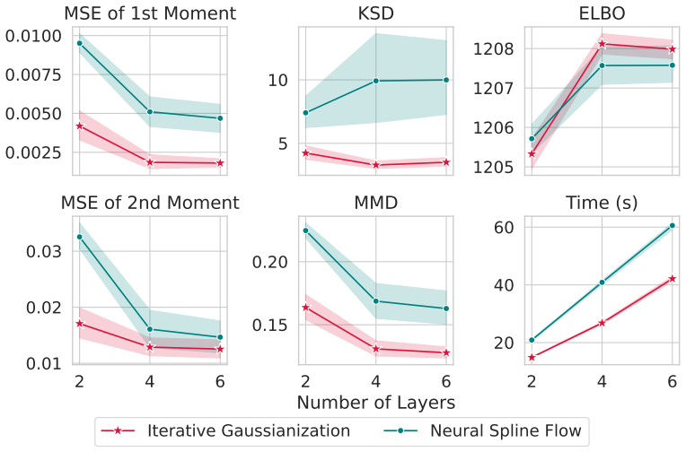
- In the reported experiments, the iterative Gaussianization matches or outperforms neural-spline-flow variational inference on several posterior sampling tasks while using a fraction of the parameters and training time.
Where Pith is reading between the lines
- A natural stress test the paper does not run: a target with strong nonlinear dependence but zero linear score cross-covariance, e.g., a symmetric mixture or a density with only quartic cross-terms in its log-density. For such a target the H-matrix would be near-zero, so the proposed rotation would offer no improvement over standard MFVI; seeing this would mark the method's boundary.
- The same rotation principle could serve as a generic preconditioning tool beyond variational inference—for example, initializing normalizing flows or choosing proposals for MCMC or sequential Monte Carlo—because it needs only the target's score at Gaussian samples, not samples from the target.
- The contraction proof for Gaussian targets uses random rotations; an analogous rate for the PCA rotation would require control of the spectral gap of H and is not in the paper. Closing that gap would put the empirical advantage of PCA rotations on the same footing as the random-rotation analysis.
Editorial analysis
A structured set of objections, weighed in public.
Referee Report
Summary. The paper proposes to enhance mean-field variational inference (MFVI) by first rotating the target distribution according to the eigenvectors of H = E_γ[x(∇log p(x)+x)^T] and then performing MFVI in the rotated coordinates. It further iterates this procedure, alternating PCA-style rotations with coordinatewise MFVI maps, to construct flow-like transport maps that push the target toward the standard Gaussian. The main theoretical results are: (i) a Gaussianity characterization via vanishing projected Fisher information under almost all rotations (Thm 3.2); (ii) a lower bound on projected Fisher information in terms of H, with equality for Gaussian targets (Thm 3.4); (iii) the optimality of the eigenvector rotation for this lower bound (Prop 4.1); and (iv) a contraction estimate for Gaussian targets under random rotations (Thm 5.2). Experiments on Bayesian logistic regression, posteriordb benchmarks, a Poisson GLMM, sparse logistic regression, and an IRT model show that PCA-rotated MFVI often improves over standard MFVI and over a small neural spline flow at comparable or lower cost.
Significance. If the claims hold, this is a practically valuable and computationally cheap way to improve MFVI, and the iterative construction offers a tractable flow-like alternative with closed-form density and inverse. The paper is transparent about the provenance of some results: Theorem 3.3 is adapted from Lacker, and the PCA objective is explicitly a lower bound. The theoretical novelty includes Theorem 3.2 and the Gaussian contraction rate, and the paper ships reproducible code. However, the theoretical support for the PCA rotation as a proxy for actual KL reduction is incomplete, and the convergence theorems apply to random rotations rather than to the PCA-based algorithm that is the paper's main recommendation. These gaps matter for the central claims and need to be addressed or carefully qualified.
major comments (3)
- [Sec. 3.3; Eq. (8)] The PCA objective maximizes a lower bound on projected Fisher information that is proven tight only for Gaussian targets (Thm 3.4). The actual MFVI improvement is the time integral of projected FI along the independent-projection dynamics (Eq. 6), or, under strong log-concavity, tilde I - J (Thm 3.3). No result shows that maximizing Σ_i(RHR^T)_ii^2 is near-optimal for Δ_MFVI, nor even that the PCA rotation improves on R=I for non-Gaussian targets. The Stein argument in §4.1 concerns infinitesimal linear perturbations, not the full nonlinear MFVI solution. Since the paper's central claim is that PCA-rotated MFVI substantially improves accuracy, the theory needs either a quantitative bound under reasonable conditions (e.g., log-concavity) or an explicit statement that the PCA selection is heuristic. The positive numerics are encouraging but do not close the gap for arbitrary non-Gaussian t
- [Sec. 5.1; Thm 5.2] The only convergence/stationarity guarantee is for rotations drawn from a full-support distribution, as explicitly assumed in the sentence 'Now suppose we draw the orthogonal matrices at random...'. The PCA-based iteration, which is the version used in Algorithm 3 and in the main experiments, has no such guarantee: it could in principle stall at a non-Gaussian distribution where the selected PCA directions yield a near-zero lower bound while a positive MFVI gap remains. Theorem 5.2 likewise assumes uniform random rotations. The conclusion that the paper has 'analyzed the algorithm' and established an entropy contraction rate therefore applies to a different rotation policy than the one recommended. Please either extend the analysis to PCA rotations or clearly delineate the theoretical results as applying to the random-rotation variant.
- [Abstract; Sec. 6.4] The claim that the method provides 'flow-like approximations ... at lower computational cost than conventional normalizing-flow variational approximations' is supported only by comparisons against a neural spline flow with one hidden layer of size 5 and 200 optimizer iterations (Sec. 6.4) and a 6-layer flow in Sec. 6.5. These are low-capacity baselines in a regime where flows are known to be at a disadvantage; the paper itself cites [1,8] showing that strong flow training requires much larger batches and careful tuning. I recommend either benchmarking against a stronger flow baseline with commensurate capacity/tuning or softening the abstract/conclusion to claim efficiency relative to flow approximations of similar capacity and training budget.
minor comments (5)
- [Fig. 1] The x-axis labels in all four panels appear to read 'd', but the caption says the right two panels vary the condition number κ. Please correct the axis labels and clarify which panels correspond to which sweep.
- [Sec. 4.1] Typo: 'the eigenvectors of of H' should be 'the eigenvectors of H'.
- [Sec. 5.1] In the display after summing over k, the averaged functional should be written as \overline{Δ_MFVI}(p^{(k-1)}); the bar is missing in the text, which makes the step from the realized sum to the averaged sum look unjustified.
- [Sec. 6.2; Table 1] The table headers use 'MF' while the text uses 'MFVI' and 'PCA-based MFVI'; make the notation consistent for readability.
- [Alg. 3] The returned transformation order is correct, but a one-line remark that this transformation maps the target to the Gaussianized distribution (and its inverse maps γ to the approximating q^{(k)}) would help the reader connect to Eq. (10).
Circularity Check
No significant circularity: the proposed rotation is derived from an independently computed target-score statistic and evaluated against external benchmarks; only minor non-load-bearing self-citations occur.
full rationale
The paper's central derivation chain is self-contained rather than circular. The rotation is chosen by maximizing the lower bound sum_i (R H R^T)^2_ii, where H = E_gamma[x(nabla log p(x)+x)^T] is an external input computed from the target density and the standard Gaussian reference. The key theoretical link between projected Fisher information and MFVI improvement is quoted from Lacker [35], an independent external source, not from the authors' own prior work. Theorem 3.4's lower bound is proven in the paper by Cauchy-Schwarz and Stein's identity, and the equality case for Gaussian targets is an additional exactness check, not an input assumption. The empirical claims are measured against NUTS reference samples and posteriordb benchmarks, so the improvement is not forced by construction. The main limitations -- the lower bound may be loose for non-Gaussian targets and the PCA-based iteration lacks the stationary guarantee that random rotations enjoy -- are performance/robustness caveats, not circular reasoning. The only self-citations are minor and non-load-bearing: [10] is cited in the literature review of mixture variational families, and [41] is mentioned in the conclusion as a possible quasi-Monte Carlo variance-reduction tool. Neither supports the paper's central premise, and no derived quantity is defined in terms of the outcome it is claimed to predict. Hence no circular step is present.
Axiom & Free-Parameter Ledger
free parameters (5)
- Principal-component retention threshold =
95% of variance explained
- Number of iterations K =
varies (e.g., 11, 4, 2/4/6)
- Monte Carlo sample size N for H estimation =
1000
- Spline knots and range boundaries =
10 knots, range (-8,8)
- Learning rate and optimizer =
Adam, lr = 0.01
axioms (6)
- domain assumption The target density p is continuously differentiable and log p, ∇log p satisfy growth conditions (finite m-th moments, polynomial growth) so the mean-field optimality equation holds.
- domain assumption The score function ∇log p(x) can be evaluated pointwise for any x, enabling Monte Carlo estimation of H and MFVI subproblems.
- domain assumption After each MFVI step, the score of the transformed target p^{(k)} can be computed to form the next H; the paper does not provide the explicit chain-rule formula but implies it is available.
- domain assumption The log-density ratio r = log(p/γ) belongs to L^2(γ) so that the Hermite polynomial expansion used in the proof of Theorem 3.2 is valid.
- domain assumption For Theorem 3.3, the potential U is strongly convex with λI ≤ ∇²U ≤ LI.
- domain assumption For Theorem 5.2, the current target is Gaussian N(0,Σ) and its mean-field approximation is already the standard Gaussian, so (Σ^{-1})_ii = 1.
read the original abstract
We propose an iterative Gaussianization method for sampling from unnormalized densities by repeatedly applying mean-field variational inference (MFVI) in rotated coordinate systems. At each iteration, the method selects a rotation, solves an MFVI subproblem in the rotated coordinates, and applies the inverse coordinatewise map to transform the current target closer to the standard Gaussian. The resulting algorithm provides a computationally efficient way to construct flow-like transport maps: it requires only MFVI subproblems, avoids large-scale optimization, and produces transformations that are easy to invert and evaluate. The effectiveness of the procedure depends on selecting informative rotations. We develop an efficient PCA-type method that chooses rotations from the leading eigenvectors of a cross-covariance matrix involving the target's score function. Experiments on Bayesian posterior sampling tasks show that performing MFVI in the proposed PCA-rotated coordinate systems substantially improves over standard MFVI, and that the resulting iterative Gaussianization procedure provides accurate flow-like approximations at lower computational cost than conventional normalizing-flow variational approximations.
Figures


Forward citations
Cited by 1 Pith paper
-
Generalized reparametrized variational Bayes with skew-symmetric normalization
KNorm-RVB combines affine normalization with mirror-reflection skewness reduction to make mean-field variational inference substantially more accurate for hierarchical models.
Reference graph
Works this paper leans on
-
[1]
and Domke, J
Agrawal, A. and Domke, J. (2025). Disentangling impact of capacity, objective, batchsize, estimators, and step-size on flow VI. InInternational Conference on Artificial Intelligence and Statistics, pages 325–333. PMLR
2025
-
[2]
Arnese, M. and Lacker, D. (2024). Convergence of coordinate ascent variational inference for log-concave measures via optimal transport.arXiv preprint arXiv:2404.08792
Pith/arXiv arXiv 2024
-
[3]
A., Salim, A., and Zhang, S
Balasubramanian, K., Chewi, S., Erdogdu, M. A., Salim, A., and Zhang, S. (2022). Towards a theory of non-log-concave sampling: first-order stationarity guarantees for Langevin Monte Carlo. InConference on Learning Theory, pages 2896–2923. PMLR
2022
-
[4]
Bhattacharya, A., Pati, D., and Yang, Y. (2025). On the convergence of coordinate ascent variational inference.The Annals of Statistics, 53(3):929–962
2025
-
[5]
Bickel, P., Choi, D., Chang, X., and Zhang, H. (2013). Asymptotic normality of maximum likelihood and its variational approximation for stochastic blockmodels.The Annals of Statistics, 41(4)
2013
-
[6]
Bishop, C. M. and Nasrabadi, N. M. (2006).Pattern Recognition and Machine Learning, volume 4. Springer
2006
-
[7]
M., Kucukelbir, A., and McAuliffe, J
Blei, D. M., Kucukelbir, A., and McAuliffe, J. D. (2017). Variational inference: A review for statisticians.Journal of the American Statistical Association, 112(518):859–877
2017
-
[8]
Blessing, D., Jia, X., Esslinger, J., Vargas, F., and Neumann, G. (2024). Beyond ELBOs: a large-scale evaluation of variational methods for sampling. InProceedings of the 41st International Conference on Machine Learning, pages 4205–4229
2024
-
[9]
D., Lee, D., Goodrich, B., Betancourt, M., Brubaker, M., Guo, J., Li, P., and Riddell, A
Carpenter, B., Gelman, A., Hoffman, M. D., Lee, D., Goodrich, B., Betancourt, M., Brubaker, M., Guo, J., Li, P., and Riddell, A. (2017). Stan: A probabilistic programming language.Journal of Statistical Software, 76:1–32
2017
-
[10]
Z., and Wang, W
Che, B., Chen, Y., Huan, Z., Huang, D. Z., and Wang, W. (2025). Stable derivative free Gaussian mixture variational inference for Bayesian inverse problems.SIAM Journal on Scientific Computing, 47(5):A2583–A2608
2025
-
[11]
and Gopinath, R
Chen, S. and Gopinath, R. (2000). Gaussianization.Advances in Neural Information Processing Systems, 13
2000
-
[12]
G., Dow, E., and Wang, Q
Constantine, P. G., Dow, E., and Wang, Q. (2014). Active subspace methods in theory and practice: applications to kriging surfaces.SIAM Journal on Scientific Computing, 36(4):A1500– A1524. 32
2014
-
[13]
M., Solonen, A., and Spantini, A
Cui, T., Martin, J., Marzouk, Y. M., Solonen, A., and Spantini, A. (2014). Likelihood-informed dimension reduction for nonlinear inverse problems.Inverse Problems, 30(11):114015
2014
-
[14]
Dinh, L., Sohl-Dickstein, J., and Bengio, S. (2017). Density estimation using Real NVP. In International Conference on Learning Representations
2017
-
[15]
Draxler, F., K¨ uhmichel, L., Rousselot, A., M¨ uller, J., Schn¨ orr, C., and K¨ othe, U. (2023). On the convergence rate of Gaussianization with random rotations. InInternational Conference on Machine Learning, pages 8449–8468. PMLR
2023
-
[16]
Du, Q., Wang, K., Zhang, E., and Zhong, C. (2024). A particle algorithm for mean-field variational inference.arXiv preprint arXiv:2412.20385
arXiv 2024
-
[17]
Durkan, C., Bekasov, A., Murray, I., and Papamakarios, G. (2019). Neural spline flows.Advances in Neural Information Processing Systems, 32
2019
-
[18]
El Moselhy, T. A. and Marzouk, Y. M. (2012). Bayesian inference with optimal maps.Journal of Computational Physics, 231(23):7815–7850
2012
-
[19]
Fong, Y., Rue, H., and Wakefield, J. (2010). Bayesian inference for generalized linear mixed models.Biostatistics, 11(3):397–412
2010
-
[20]
and Tukey, J
Friedman, J. and Tukey, J. (1974). A projection pursuit algorithm for exploratory data analysis. IEEE Transactions on Computers, 100(SLAC-PUB-1312)
1974
-
[21]
Friedman, J. H. (1987). Exploratory projection pursuit.Journal of the American Statistical Association, 82(397):249–266
1987
-
[22]
M., and Vanden-Eijnden, E
Gabri´ e, M., Rotskoff, G. M., and Vanden-Eijnden, E. (2022). Adaptive Monte Carlo augmented with normalizing flows.Proceedings of the National Academy of Sciences, 119(10):e2109420119
2022
-
[23]
and Mackey, L
Gorham, J. and Mackey, L. (2015). Measuring sample quality with Stein’s method.Advances in Neural Information Processing Systems, 28
2015
-
[24]
Han, S., Liao, X., Dunson, D., and Carin, L. (2016). Variational Gaussian copula inference. In Artificial Intelligence and Statistics, pages 829–838. PMLR
2016
-
[25]
Hastings, W. K. (1970). Monte Carlo sampling methods using Markov chains and their applications.Biometrika, 57(1):97
1970
-
[26]
V., Langmore, I., Tran, D., and Vasudevan, S
Hoffman, M., Sountsov, P., Dillon, J. V., Langmore, I., Tran, D., and Vasudevan, S. (2019). Neutra-lizing bad geometry in Hamiltonian Monte Carlo using neural transport.arXiv preprint arXiv:1903.03704
Pith/arXiv arXiv 2019
-
[27]
Hoffman, M. D. and Gelman, A. (2014). The No-U-Turn sampler: adaptively setting path lengths in Hamiltonian Monte Carlo.J. Mach. Learn. Res., 15(1):1593–1623
2014
-
[28]
Hofmann, H. (1994). Statlog (German Credit Data). UCI Machine Learning Repository. DOI: https://doi.org/10.24432/C5NC77
doi:10.24432/c5nc77 1994
-
[29]
Huber, P. J. (1985). Projection pursuit.The Annals of Statistics, pages 435–475
1985
-
[30]
Jiang, Y., Chewi, S., and Pooladian, A.-A. (2025). Algorithms for mean-field variational inference via polyhedral optimization in the Wasserstein space.Foundations of Computational Mathematics, pages 1–52. 33
2025
-
[31]
I., Ghahramani, Z., Jaakkola, T
Jordan, M. I., Ghahramani, Z., Jaakkola, T. S., and Saul, L. K. (1999). An introduction to variational methods for graphical models.Machine learning, 37(2):183–233
1999
-
[32]
Kingma, D. P. (2014). Adam: A method for stochastic optimization.arXiv preprint arXiv:1412.6980
Pith/arXiv arXiv 2014
-
[33]
P., Salimans, T., Jozefowicz, R., Chen, X., Sutskever, I., and Welling, M
Kingma, D. P., Salimans, T., Jozefowicz, R., Chen, X., Sutskever, I., and Welling, M. (2016). Improved variational inference with inverse autoregressive flow.Advances in Neural Information Processing Systems, 29
2016
-
[34]
Kotz, S., Balakrishnan, N., and Johnson, N. L. (2019).Continuous Multivariate Distributions, Volume 1: Models and Applications, volume 1. John Wiley & Sons
2019
-
[35]
Lacker, D. (2023). Independent projections of diffusions: Gradient flows for variational inference and optimal mean field approximations.arXiv preprint arXiv:2309.13332
Pith/arXiv arXiv 2023
-
[36]
Lacker, D., Mukherjee, S., and Yeung, L. C. (2024). Mean field approximations via log-concavity. International Mathematics Research Notices, 2024(7):6008–6042
2024
-
[37]
Laparra, V., Camps-Valls, G., and Malo, J. (2011). Iterative Gaussianization: from ICA to random rotations.IEEE Transactions on Neural Networks, 22(4):537–549
2011
-
[38]
and Zanella, G
Lavenant, H. and Zanella, G. (2024). Convergence rate of random scan coordinate ascent variational inference under log-concavity.SIAM Journal on Optimization, 34(4):3750–3761
2024
-
[39]
E., and Schmidt, M
Lin, W., Khan, M. E., and Schmidt, M. (2019). Fast and simple natural-gradient variational inference with mixture of exponential-family approximations. InInternational Conference on Machine Learning, pages 3992–4002. PMLR
2019
-
[40]
and Wang, D
Liu, Q. and Wang, D. (2016). Stein variational gradient descent: A general purpose Bayesian inference algorithm.Advances in Neural Information Processing Systems, 29
2016
-
[41]
Liu, S. (2024). Transport quasi-Monte Carlo.arXiv preprint arXiv:2412.16416
Pith/arXiv arXiv 2024
-
[42]
Magnusson, M., Torgander, J., B¨ urkner, P.-C., Zhang, L., Carpenter, B., and Vehtari, A. (2024). posteriordb: Testing, benchmarking and developing Bayesian inference algorithms. InThe 28th International Conference on Artificial Intelligence and Statistics
2024
-
[43]
Meng, C., Song, Y., Song, J., and Ermon, S. (2020). Gaussianization flows. InInternational Conference on Artificial Intelligence and Statistics, pages 4336–4345. PMLR
2020
-
[44]
W., Rosenbluth, M
Metropolis, N., Rosenbluth, A. W., Rosenbluth, M. N., Teller, A. H., and Teller, E. (1953). Equation of state calculations by fast computing machines.The Journal of Chemical Physics, 21(6):1087–1092
1953
-
[45]
E., Ormerod, J
Neville, S. E., Ormerod, J. T., and Wand, M. (2014). Mean field variational Bayes for continuous sparse signal shrinkage: Pitfalls and remedies.Electronic Journal of Statistics, 8:1113–1151
2014
-
[46]
and Archambeau, C
Opper, M. and Archambeau, C. (2009). The variational Gaussian approximation revisited. Neural computation, 21(3):786–792
2009
-
[47]
Papamakarios, G. et al. (2021). Normalizing flows for probabilistic modeling and inference. Journal of Machine Learning Research, 22(57):1–64
2021
-
[48]
O., and Sk¨ old, M
Papaspiliopoulos, O., Roberts, G. O., and Sk¨ old, M. (2007). A general framework for the parametrization of hierarchical models.Statistical Science, pages 59–73. 34
2007
-
[49]
Parno, M. D. and Marzouk, Y. M. (2018). Transport map accelerated Markov chain Monte Carlo.SIAM/ASA Journal on Uncertainty Quantification, 6(2):645–682
2018
-
[50]
and Mohamed, S
Rezende, D. and Mohamed, S. (2015). Variational inference with normalizing flows. In International conference on machine learning, pages 1530–1538. PMLR
2015
-
[51]
Sklar, M. (1959). Fonctions de r´ epartition ` a n dimensions et leurs marges. InAnnales de l’ISUP, volume 8, pages 229–231
1959
-
[52]
https://mc-stan.org/docs/ stan-users-guide/regression.html#multilevel-2pl-model
Stan Development Team (2011).Stan User’s Guide. https://mc-stan.org/docs/ stan-users-guide/regression.html#multilevel-2pl-model
2011
-
[53]
Tabak, E. G. and Turner, C. V. (2013). A family of nonparametric density estimation algorithms. Communications on Pure and Applied Mathematics, 66(2):145–164
2013
-
[54]
Tabak, E. G. and Vanden-Eijnden, E. (2010). Density estimation by dual ascent of the log-likelihood.Communications in Mathematical Sciences, 8(1):217–233
2010
-
[55]
Tan, L. S. (2021). Use of model reparametrization to improve variational Bayes.Journal of the Royal Statistical Society Series B: Statistical Methodology, 83(1):30–57
2021
-
[56]
Tran, M.-N., Tseng, P., and Kohn, R. (2023). Particle mean field variational Bayes.arXiv preprint arXiv:2303.13930
Pith/arXiv arXiv 2023
-
[57]
Wainwright, M. J. and Jordan, M. I. (2008). Graphical models, exponential families, and variational inference.Foundations and Trends®in Machine Learning, 1(1–2):1–305
2008
-
[58]
and Titterington, D
Wang, B. and Titterington, D. M. (2005). Inadequacy of interval estimates corresponding to variational Bayesian approximations. InInternational Workshop on Artificial Intelligence and Statistics, pages 373–380. PMLR
2005
-
[59]
Zahm, O., Cui, T., Law, K., Spantini, A., and Marzouk, Y. (2022). Certified dimension reduction in nonlinear Bayesian inverse problems.Mathematics of Computation, 91(336):1789–1835
2022
-
[60]
´A., Jaitly, N., and Susskind, J
Zhai, S., Zhang, R., Nakkiran, P., Berthelot, D., Gu, J., Zheng, H., Chen, T., Bautista, M. ´A., Jaitly, N., and Susskind, J. M. (2025). Normalizing flows are capable generative models. In Forty-second International Conference on Machine Learning
2025
-
[61]
and Gao, C
Zhang, F. and Gao, C. (2020). Convergence rates of variational posterior distributions.The Annals of Statistics, 48(4):2180–2207
2020
-
[62]
and Yang, Y
Zhang, Y. and Yang, Y. (2024). Bayesian model selection via mean-field variational approximation.Journal of the Royal Statistical Society Series B: Statistical Methodology, 86(3):742– 770. 35
2024
discussion (0)
Sign in with ORCID, Apple, or X to comment. Anyone can read and Pith papers without signing in.