Post-selection inference for penalized M-estimators via score thinning

Daniela Witten; Ronan Perry; Snigdha Panigrahi

REVIEW 3 major objections 4 minor 1 cited by

Ordinary confidence intervals can be made valid after model selection by splitting a score variable with noise.

Reviewed by Pith at T0; open to challenge. T0 means a machine referee read the full paper against a public rubric. the ladder, T0–T4 →

Challenge this review Re-run · record.json Download PDF Read on arXiv ↗

T0 review · deepseek-v4-flash

2026-08-03 09:30 UTC pith:MWZBYCNR

load-bearing objection Score-thinning is a real advance, but the theory and simulations operate in different asymptotic regimes—still worth a serious referee. the 3 major comments →

arxiv 2601.13514 v2 pith:MWZBYCNR submitted 2026-01-20 stat.ME

Post-selection inference for penalized M-estimators via score thinning

Ronan Perry , Snigdha Panigrahi , Daniela Witten This is my paper

classification stat.ME MSC 62J0762F1262E20

keywords post-selection inferenceselective inferencepenalized M-estimationscore variabledata splittingrandomized lassoconfidence intervalsasymptotic coverage

verification ladder T0 review T1 audit T2 compute T3 formal T4 reserved

The pith

A machine-rendered reading of the paper's core claim, the machinery that carries it, and where it could break.

This paper claims that post-selection inference for penalized M-estimators does not require bespoke selective-inference pipelines. The key observation is that both the event that a penalized M-estimator selects a given model and the event that a standard confidence interval covers its target can be expressed as events involving one approximately normal score variable. If that score is split into two approximately independent pieces by adding and subtracting carefully scaled Gaussian noise, the selection event and the coverage event become asymptotically independent. As a result, standard confidence intervals centered on a noisy estimator attain the nominal coverage conditional on the selected model. The paper works out the theory for fixed p and growing n, and shows it holds for generalized linear models, where comparable thinning methods do not apply.

Core claim

The central claim is Theorem 6: under regularity conditions, a standard (non-selective) confidence interval centered at the noisy model-E M-estimator covers the population parameter conditional on the event that the noisy penalized M-estimator selected model E, with asymptotic probability at least 1-alpha. The proof decomposes the score variable into two approximately independent normal variables, shows the selection event depends only on one piece (up to a vanishing remainder) via the KKT conditions, and the coverage event only on the other, then applies a conditional Berry-Esseen bound. Corollary 7 extends the result to adding noise directly to the outcomes whenever the loss is affine in t

What carries the argument

The score variable Zhat_n = sqrt(n) P_n \dot ell_{theta-bar_n^{E,*}}, the normalized gradient of the loss at the population parameter of the selected model. Gaussian thinning: with W ~ N(0, Sigma-hat), set Z^(1) = Zhat + gamma W and Z^(2) = Zhat - (1/gamma) W; these are approximately independent normals. The selection event equals {Z^(1) + o_p(1) in a union of convex sets} (Lemma 4), and the coverage event equals {Z^(2) + o_p(1) in a convex set} (Lemma 5). Lemma 2's conditional Berry-Esseen bound converts this approximate independence into a conditional-coverage guarantee in Theorem 6.

Load-bearing premise

The loss function's gradient must admit a uniform second-order Taylor expansion around the selected-model parameter whose remainder is o_p(n^{-1/2}); if that quick decay fails, both the event characterizations and the coverage guarantee collapse.

What would settle it

Simulate a setting where the Taylor remainder is not o_p(n^{-1/2}) (for example, median regression with fixed p and n) and measure the conditional coverage of the proposed interval; a persistent gap below 1-alpha would refute the theorem's reach. Alternatively, check whether Condition 4 holds for a given loss by verifying the remainder rate directly.

Watch this falsifier — get emailed when new claim-graph text bears on it.

If this is right

For practitioners, valid post-selection inference after lasso-style selection reduces to fitting two M-estimators, one with noise added and one with noise subtracted; no special selective-inference software is required.
The result covers generalized linear models with canonical links, including logistic regression, a setting where exact data-thinning methods are unavailable.
Coverage is conditional on the selected model, not merely unconditional, so the guarantee is the one selective-inference users actually want.
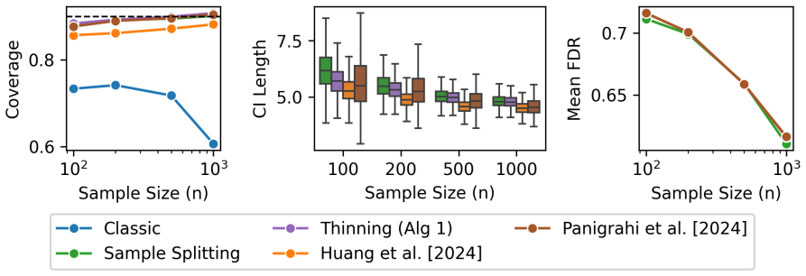
Intervals from this approach are wider than those from exact randomized selective inference in simulations, but narrower than sample splitting, offering a trade-off between convenience and power.
Corollary 7 implies that for appropriate losses, the analyst may add noise to the response instead of to the optimization objective, which is computationally simpler.

Where Pith is reading between the lines

These are editorial extensions of the paper, not claims the author makes directly.

Editorial inference: the same score-splitting mechanism could plausibly be adapted to provide valid post-selection p-values and false-discovery-rate control, not just confidence intervals, for penalized M-estimators.
Editorial inference: Condition 5 restricts the approach to penalties whose selection regions are finitely piecewise-convex (true for the lasso but open for the group lasso); extending it would cover more structured penalties.
Editorial inference: a promising stress test is the p > n regime, which the paper leaves open; score thinning may behave differently when the score covariance is singular.
Editorial inference: the asymptotic independence between selection and inference suggests that the variance estimator and the noise split gamma could be tuned separately, hinting at a possible power-improving modification.

Editorial analysis

A structured set of objections, weighed in public.

Desk editor's note, referee report, simulated authors' rebuttal, and a circularity audit.

Desk Editor's Note

Score-thinning is a real advance, but the theory and simulations operate in different asymptotic regimes—still worth a serious referee.

read the letter

Dear colleague,

The headline is this: the score-thinning construction is a genuine step forward in post-selection inference, and the central theorem is probably right under its stated assumptions—but the experiments are run in a regime the theorem doesn't cover, and the paper doesn't say so.

What's new: rather than deriving a bespoke selective distribution for each penalty, the authors show that if you add carefully chosen Gaussian noise to the score (or, for GLMs, to the outcomes), the model selection event and the coverage event of a standard CI can both be written as events involving two approximately independent normal score variables. That lets you use ordinary software for the whole pipeline. The construction is clean, and it extends the thinning idea to logistic regression and cluster-correlated data, where previous data-thinning/fission results didn't apply. The proofs are detailed; Lemmas 4–5 and Theorem 6 have a real Berry-Esseen argument, and I didn't find a hole in that reasoning.

Where it's soft. The biggest issue is that Theorem 6 relies on Assumption 1(i), a local-alternative condition that keeps the selection event non-degenerate in the limit. The simulations and the network application use a fixed sparse truth, so sqrt(n) θ^{E,*}_n blows up. In that case the selection probability for any given wrong model goes to zero, the denominator in Lemma 2 isn't bounded away from zero, and the proof of Theorem 6 doesn't apply. The paper acknowledges the local-alternative assumption when it introduces it, but never flags that its own empirical section doesn't live in that regime. That's a real mismatch, and it should be addressed—either by a theory for fixed alternatives (or at least a heuristic argument) or by a clear statement that the simulations are a sanity check rather than a confirmation of the theorem.

Second, Condition 3 is assumed rather than proved in general. For GLMs they show it holds, but the theorem statement would be cleaner if they gave a general sufficient condition. Relatedly, the proof of Theorem 6 needs consistency of Ŝ^E_n, which isn't stated in Assumption 1. These are fixable.

The paper is honestly written, with limitations (n>p, L1-only) disclosed. I'd send it to a referee. It deserves one.

All best.

Referee Report

3 major / 4 minor

Summary. This paper proposes a method for post-selection inference after penalized M-estimation. The main idea is to add Gaussian noise to the score of an M-estimator and use the two resulting noisy score variables for selection and inference, respectively. Under regularity conditions, the authors show that the selection event and the event that a standard fixed-model confidence interval covers its target can both be approximately characterized by these thinned score variables, yielding asymptotic conditional coverage (Theorem 6). A corollary applies the result to generalized linear models by adding noise directly to the outcomes (Corollary 7). The paper includes a Berry--Esseen-type analysis, simulation studies in linear, logistic, and cluster-correlated settings, and an application to a social network.

Significance. If the main theorem is correct, this is a substantial contribution: it would provide a simple, distribution-free, asymptotically valid alternative to bespoke selective inference procedures for a broad class of penalized M-estimators. The paper builds on and extends data-thinning ideas, and the proof machinery—especially the conditional Berry--Esseen bound—is nontrivial and largely carefully developed. The authors also provide code, which is valuable for reproducibility. However, as detailed below, the theorem is proved only under a local-alternative assumption that the paper's own simulations and application do not satisfy, and the proof has a gap concerning convergence of the variance estimator. The conceptual promise is real, but the current manuscript needs additional work before the central claim can be regarded as fully established.

major comments (3)

[Assumption 1(i) and Section 5.1] Please note the above comment is the same as the intended comment; the section field is used for citation.
[Appendix B.5 (proof of Theorem 6)] This is a separate technical issue from the local-alternative mismatch.
[Algorithm 1, Step 2] This issue is local but affects the empirical implementation.

minor comments (4)

[Abstract and general presentation] There are several typographical issues, e.g., "independen" in the abstract and formatting glitches like "glmnetinR". A careful proofread is recommended.
[Section 3.2, Corollary 7] The condition \ell_\theta(Y_i) = \theta^T A_i Y_i + a_{\theta,i} is stated with A_i of dimension p x d. In the GLM application, Y_i is scalar and A_i = -X_i, so A_i \bar W_{n,i} is p-dimensional. This is clear enough, but it would help to explicitly state the dimensions in Section 3.2 to avoid confusion.
[Section 5.1] The sentence "We note the following." and the list formatting could be improved. Also, the claim that "All other approaches attain 90% coverage" is contradicted by the displayed undercoverage of Huang et al. in Figure 1; the text should be clarified.
[Section 6] The discussion lists limitations n > p and L1-only penalty, but as noted above it does not mention the local-alternative restriction or the lack of validation in that regime. The discussion would be more transparent if this were included.

Circularity Check

0 steps flagged

No circularity: the conditional coverage result is derived, not assumed, and self-citations are background building blocks.

full rationale

The central claim, Theorem 6, is that a standard non-selective confidence interval attains nominal coverage conditional on the model selected by a noisy penalized M-estimator. The proof does not assume this conditional coverage. Its inputs are: (i) approximate Gaussianity of the score variable (Condition 1, Lemma 1); (ii) a conditional Berry-Esseen bound that measures how close conditional probabilities are to unconditional ones (Lemma 2); (iii) a characterization of the selection and coverage events as convex-set events in thinned score variables (Lemmas 4 and 5); and (iv) Condition 3, which is only the fixed-model, non-selective coverage of the same interval. The target conditional coverage is then obtained by showing the difference between conditional and unconditional coverage vanishes. The construction of the thinned scores (2.10) borrows the adding/subtracting-noise idea from the data-thinning literature (Rasines and Young 2023; Neufeld et al. 2024; Dharamshi et al. 2025), but the paper proves its own Berry-Esseen-type bounds and does not import a post-selection theorem from those citations. The self-citations (Neufeld, Dharamshi, Witten; Panigrahi) are background references and are not load-bearing in the proof of Theorem 6. The local-alternative Assumption 1(i) is a genuine technical condition, and the reviewer's observation that the simulations use fixed sparse parameters is a real concern about the scope of the experiments, but it is a mismatch between assumptions and simulations, not a circular derivation. Similarly, the Discussion's stated limitations (n > p, L1-only verification) are honest scope restrictions, not hidden circular inputs. Therefore the derivation chain is self-contained relative to its stated assumptions, and no step reduces by definition to its own output.

Axiom & Free-Parameter Ledger

2 free parameters · 10 axioms · 0 invented entities

The method introduces no new scientific entities, particles, or forces. It relies on a list of standard but nontrivial regularity conditions (Conditions 1–7, Assumption 1) and two user-chosen tuning parameters, γ and λ. The most honesty-relevant item is Condition 3, which is an assumed property of a standard CI rather than something derived in full generality; for GLMs the paper sketches a sandwich-estimator justification.

free parameters (2)

γ (information split) = γ=1 in experiments
User-chosen noise-splitting ratio; controls variance allocation between selection and inference; not fitted to data but load-bearing for the method.
λ (penalty strength) = λ∝√(log p)·sd(Y) in simulations and application
Lasso penalty scale used in (3.4)/(3.1); chosen by formula, not optimized for coverage.

axioms (10)

domain assumption Observations are independent (triangular array), not necessarily i.i.d.
Section 2.1: Y_i ind.∼ F_n; needed for Berry-Esseen bounds and asymptotic independence.
domain assumption Condition 1: score covariance Σ_n is invertible and centered third moments are uniformly bounded
Required for the approximate normality of the score variable and for Lemma 1/Lemma 2.
domain assumption Condition 2: uniqueness of the penalized estimator and submodel estimator
Used in Lemma 4 to characterize the selection event exactly via KKT conditions.
domain assumption Condition 3: existence of a standard fixed-model CI around the noisy M-estimator with asymptotic coverage
This is the non-selective benchmark whose coverage is transferred to the conditional guarantee by Theorem 6.
domain assumption Condition 4: uniform second-order Taylor expansion of the score with o_p(n^{-1/2}) remainder for both estimators
Bridges the KKT/coverage events to thinned score variables in Lemmas 4 and 5; the load-bearing regularity condition.
domain assumption Assumption 1: local alternatives and convergence of Σ_n and H_n
Ensures selection probability does not vanish asymptotically and that the sets A^E_n, B^E_n stabilize for Lemma 2's denominator lower bound.
domain assumption Condition 5: penalty subgradient sets form finite unions of convex sets with nonempty interiors
Used to write the selection event as a union of convex sets; proven for the L1 penalty in Proposition 3.
domain assumption Condition 6: L1 consistency of the score covariance estimator
Controls the error from replacing the true covariance with an estimate when thinning the score.
domain assumption Condition 7: loss is affine in the response with fixed matrices A_i
Allows noise to be added to outcomes rather than directly to the score; satisfied by GLMs with canonical links.
domain assumption p is fixed and n→∞
Explicitly stated as a limitation in Section 6; all theory is in this regime.

pith-pipeline@v1.3.0-alltime-deepseek · 35920 in / 17766 out tokens · 168040 ms · 2026-08-03T09:30:43.070363+00:00 · methodology

0 comments

read the original abstract

We consider inference for M-estimators after model selection using a sparsity-inducing penalty. While existing methods for this task require bespoke inference procedures, we propose a simpler approach, which relies on two insights: (i) adding and subtracting carefully-constructed noise to a Gaussian random variable with unknown mean and known variance leads to two \emph{independent} Gaussian random variables; and (ii) both the selection event resulting from penalized M-estimation, and the event that a standard (non-selective) confidence interval for an M-estimator covers its target, can be characterized in terms of an approximately normal ``score variable". We combine these insights to show that -- when the noise is chosen carefully -- there is asymptotic independence between the model selected using a noisy penalized M-estimator, and the event that a standard (non-selective) confidence interval on noisy data covers the selected parameter. Therefore, selecting a model via penalized M-estimation (e.g. \verb=glmnet= in \verb=R=) on noisy data, and then conducting \emph{standard} inference on the selected model (e.g. \verb=glm= in \verb=R=) using noisy data, yields valid inference: \emph{no bespoke methods are required}. Our results require independence of the observations, but only weak distributional requirements. We apply the proposed approach to conduct inference on the association between sex and smoking in a social network.

Figures

Figures reproduced from arXiv: 2601.13514 by Daniela Witten, Ronan Perry, Snigdha Panigrahi.

**Figure 2.** Figure 2: We simulate outcomes from a logistic regression model. Inference is conducted [PITH_FULL_IMAGE:figures/full_fig_p022_2.png] view at source ↗

**Figure 3.** Figure 3: Outcomes are generated from a linear model with equicorrelated non-Gaussian [PITH_FULL_IMAGE:figures/full_fig_p022_3.png] view at source ↗

**Figure 4.** Figure 4: (Left): the friendship network of students, colored by recorded sex. (Middle): [PITH_FULL_IMAGE:figures/full_fig_p024_4.png] view at source ↗

discussion (0)

Forward citations

Cited by 1 Pith paper

Reviewed papers in the Pith corpus that reference this work. Sorted by Pith novelty score.

Flexible Inference for Winners with Conditional Validity
stat.ME 2026-07 conditional novelty 6.0

A data-adaptive exponential randomization scheme yields conditionally valid confidence intervals for top-k winners, with selection quality close to standard top-k and shorter intervals than polyhedral methods.

Reference graph

Works this paper leans on

6 extracted references · cited by 1 Pith paper

[1]

˜θn ←arg min θ∈Rp Pnℓθ
[2]

Sample noise ˆWn ←N 0, 1 n Pn i=1 Xi ¨b X ⊤ i ˜θn X ⊤ i /α ˜θn
[3]

Estimate ˆθ(λ) n as in (3.1) and defineE:= supp ˆθ(λ) n
[4]

Estimate ˆθE n as in (3.5)
[5]

the form 1 n nX i=1 Yi − 1 γ ˜Wn,i − ˙b(X ⊤ i,E ˆθE n ) 2 Xi,EX ⊤ i,E

Compute the modified sandwich variance estimator: ˆSE n ← Hn,E,E ˆθE n −1 ˜Σn,E,E Hn,E,E ˆθE n −1 where ˜Σn,E,E ← 1 γ2 Var ˆWn,E,E + 1 n nX i=1 Yi − ˙b(X ⊤ i,E ˆθE n ) 2 Xi,EX ⊤ i,E.(C.1) Output:A confidence interval centered at ˆθE n , CIξ,α n ˆθE n , ˆSE n = ξ⊤ ˆθE n ±n −1/2z1−α/2 ξ⊤ ˆSE n ξ 1/2 . the form 1 n nX i=1 Yi − 1 γ ˜Wn,i − ˙b(X ⊤ i,E ˆθE n ) ...
[2023]

To apply this result to ˆWn andW n, we must condition on ˆΣn so that ˆWn is Gaussian

allows us to bound the total variation between two Gaussian random variables with the same mean but different covariances. To apply this result to ˆWn andW n, we must condition on ˆΣn so that ˆWn is Gaussian. Since ˆΣn is a function of the data Dn :={(X i, Yi)}n i=1, it is sufficient to condition onD n. By Theorem 1.1 and Equation 2 of Devroye et al. [202...

2023

[1] [1]

˜θn ←arg min θ∈Rp Pnℓθ

[2] [2]

Sample noise ˆWn ←N 0, 1 n Pn i=1 Xi ¨b X ⊤ i ˜θn X ⊤ i /α ˜θn

[3] [3]

Estimate ˆθ(λ) n as in (3.1) and defineE:= supp ˆθ(λ) n

[4] [4]

Estimate ˆθE n as in (3.5)

[5] [5]

the form 1 n nX i=1 Yi − 1 γ ˜Wn,i − ˙b(X ⊤ i,E ˆθE n ) 2 Xi,EX ⊤ i,E

Compute the modified sandwich variance estimator: ˆSE n ← Hn,E,E ˆθE n −1 ˜Σn,E,E Hn,E,E ˆθE n −1 where ˜Σn,E,E ← 1 γ2 Var ˆWn,E,E + 1 n nX i=1 Yi − ˙b(X ⊤ i,E ˆθE n ) 2 Xi,EX ⊤ i,E.(C.1) Output:A confidence interval centered at ˆθE n , CIξ,α n ˆθE n , ˆSE n = ξ⊤ ˆθE n ±n −1/2z1−α/2 ξ⊤ ˆSE n ξ 1/2 . the form 1 n nX i=1 Yi − 1 γ ˜Wn,i − ˙b(X ⊤ i,E ˆθE n ) ...

[6] [2023]

To apply this result to ˆWn andW n, we must condition on ˆΣn so that ˆWn is Gaussian

allows us to bound the total variation between two Gaussian random variables with the same mean but different covariances. To apply this result to ˆWn andW n, we must condition on ˆΣn so that ˆWn is Gaussian. Since ˆΣn is a function of the data Dn :={(X i, Yi)}n i=1, it is sufficient to condition onD n. By Theorem 1.1 and Equation 2 of Devroye et al. [202...

2023