Online Conformal Prediction with Adversarial Semi-bandit Feedback via Regret Minimization
Pith reviewed 2026-05-10 05:04 UTC · model grok-4.3
The pith
Online conformal prediction with partial feedback achieves long-run coverage by linking it to adversarial bandit regret.
A machine-rendered reading of the paper's core claim, the machinery that carries it, and where it could break.
Core claim
We formulate online conformal prediction as an adversarial bandit problem by treating each candidate prediction set as an arm. Building on an existing algorithm for adversarial bandits, our method achieves a long-run coverage guarantee by explicitly establishing its connection to the regret of the learner.
What carries the argument
Reduction of conformal set selection to adversarial semi-bandit regret minimization, where each possible prediction set is an arm and feedback arrives only on the chosen arm when the label lies inside it.
If this is right
- The miscoverage rate converges to the desired level in the long run without any distributional assumptions on the data.
- Prediction sets of controlled average size can be produced online even though full labels are never observed.
- The same regret bound applies in both i.i.d. and non-i.i.d. sequences, including adversarial ones.
- Any improvement in the underlying adversarial bandit algorithm directly tightens the coverage guarantee.
Where Pith is reading between the lines
- The regret connection suggests that faster-regret bandit methods could shrink prediction sets without sacrificing coverage.
- The semi-bandit model may apply directly to active-learning or costly-label streams where only uncertain points receive labels.
- One could test whether the same reduction yields finite-time coverage bounds rather than only asymptotic ones.
Load-bearing premise
The true label is revealed exactly when it lies inside the constructed prediction set, and the adversary is adaptive but the feedback model remains semi-bandit.
What would settle it
Run the algorithm for many steps against an adaptive adversary that forces miscoverage whenever possible under the semi-bandit rule; if the long-run miscoverage rate exceeds the target level by more than a constant factor, the claimed guarantee fails.
Figures




read the original abstract
Uncertainty quantification is crucial in safety-critical systems, where decisions must be made under uncertainty. In particular, we consider the problem of online uncertainty quantification, where data points arrive sequentially. Online conformal prediction is a principled online uncertainty quantification method that dynamically constructs a prediction set at each time step. While existing methods for online conformal prediction provide long-run coverage guarantees without any distributional assumptions, they typically assume a full feedback setting in which the true label is always observed. In this paper, we propose a novel learning method for online conformal prediction with partial feedback from an adaptive adversary-a more challenging setup where the true label is revealed only when it lies inside the constructed prediction set. Specifically, we formulate online conformal prediction as an adversarial bandit problem by treating each candidate prediction set as an arm. Building on an existing algorithm for adversarial bandits, our method achieves a long-run coverage guarantee by explicitly establishing its connection to the regret of the learner. Finally, we empirically demonstrate the effectiveness of our method in both independent and identically distributed (i.i.d.) and non-i.i.d. settings, showing that it successfully controls the miscoverage rate while maintaining a reasonable size of the prediction set.
Editorial analysis
A structured set of objections, weighed in public.
Referee Report
Summary. The manuscript proposes a method for online conformal prediction under adversarial semi-bandit feedback, where the true label is revealed only if it falls inside the constructed prediction set. It formulates the problem as an adversarial bandit by treating candidate prediction sets as arms, applies an existing no-regret algorithm, and derives a long-run coverage guarantee (miscoverage at most alpha plus sublinear regret) from the connection to the learner's regret against the best fixed arm in hindsight. The 0-1 miscoverage loss is treated as observable under the given feedback model. Empirical results are reported for both i.i.d. and non-i.i.d. settings.
Significance. If the regret connection holds, this provides a clean theoretical extension of online conformal prediction to partial-feedback settings that arise in many practical applications. The explicit reduction to standard adversarial bandit regret bounds (with the (1-alpha)-quantile arm as comparator) is a strength, as is the absence of distributional assumptions. The empirical validation across data regimes adds relevance, though limited baseline and variance details reduce the strength of the practical claims.
minor comments (2)
- [Empirical Evaluation] Empirical Evaluation section: the description of baselines is insufficient; it is unclear which prior online conformal prediction methods are used for comparison and how they are modified for the semi-bandit feedback model.
- [Empirical Evaluation] Empirical Evaluation section: no standard deviations, confidence intervals, or multiple-run statistics are reported for the miscoverage rates and average set sizes, which weakens assessment of result stability.
Simulated Author's Rebuttal
We thank the referee for their positive summary of the manuscript, recognition of the clean reduction to adversarial bandit regret, and recommendation for minor revision. We address the concern raised in the significance assessment below.
read point-by-point responses
-
Referee: limited baseline and variance details reduce the strength of the practical claims
Authors: We agree that the empirical section would benefit from additional baselines and variability reporting. In the revised manuscript we will add comparisons against simple baselines (e.g., always outputting the full label space and a fixed-size quantile set) and report mean performance together with standard deviations across at least ten independent random seeds for both the i.i.d. and non-i.i.d. regimes. These changes will strengthen the practical claims while leaving the theoretical results unchanged. revision: yes
Circularity Check
No significant circularity in the derivation chain
full rationale
The paper models online conformal prediction under semi-bandit feedback by treating candidate prediction sets as arms in an adversarial bandit problem, with the 0-1 miscoverage loss directly observable from whether the label is revealed. It invokes an existing no-regret algorithm for adversarial bandits and derives the long-run coverage guarantee from the standard regret bound relative to the best fixed arm in hindsight. The comparator arm is defined as the (1-alpha)-quantile arm whose hindsight miscoverage equals alpha, so the average loss bound directly yields the desired guarantee without any self-referential fitting, ansatz smuggling, or load-bearing self-citation. The reduction relies on external bandit theory applied to the explicitly observable loss, making the derivation self-contained against the stated assumptions.
Axiom & Free-Parameter Ledger
axioms (2)
- standard math Standard regret bounds hold for the chosen adversarial bandit algorithm under adaptive adversaries.
- domain assumption The feedback model is exactly semi-bandit: label observed iff inside the chosen prediction set.
Forward citations
Cited by 1 Pith paper
-
Online Conformal Prediction for Non-Exchangeable Panel Data
An online conformal prediction framework for non-exchangeable panel data that forms prediction sets using related units' contemporaneous data with adaptive similarity weights and miscoverage levels to deliver stepwise...
Reference graph
Works this paper leans on
-
[1]
Haosen Ge, Hamsa Bastani, and Osbert Bastani
Accessed: 2025-09-22. Haosen Ge, Hamsa Bastani, and Osbert Bastani. Stochastic Online Conformal Prediction with Semi-bandit Feedback. InICML,
work page 2025
-
[2]
Language Models with Conformal Factuality Guaran- tees
11 Published as a conference paper at ICLR 2026 Christopher Mohri and Tatsunori Hashimoto. Language Models with Conformal Factuality Guaran- tees. InICML,
work page 2026
-
[3]
12 Published as a conference paper at ICLR 2026 A PRELIMINARY A.1 ADVERSARIALBANDITPROBLEM The multi-armed bandit problem is a sequential game between a learner and an environment (Slivkins, 2019; Lattimore & Szepesvári, 2020), where the game proceeds over T∈N rounds. At each round t∈[T] , the learner chooses an arm πt from a given set Π, where we refer t...
work page 2026
-
[4]
by controlling the variance of regret. Theorem 2(Auer et al. (2002)).For any δ∈(0,1) and ℓt(π)∈[ℓ min, ℓmax], run EXP3.P (Algo- rithm
work page 2002
-
[5]
with β= q lnK KT , γ= 1.05 q KlnK T ,andη= 0.95 q lnK KT . Then, with probability at least 1−δ, the regretReg(T)satisfies Reg(T)≤(ℓ max −ℓ min) r T K lnK ln(δ−1) + 5.15 √ T KlnK ! . Algorithm 2EXP3.P 1:procedureEXP3.P(Π, T, η, γ, β) 2:Initialize cumulative estimated gain: ˜G0(π)←0for allπ∈Π 3:fort∈ {1, . . . , T}do 4:Update strategy:p t(π)←(1−γ) exp(η ˜Gt...
work page 2026
-
[6]
T Cgap(T)o(T) −1 | {z } CMC(T) . 15 Published as a conference paper at ICLR 2026 CEXP3.P-STYLEALGORITHMS FORONLINECONFORMALPREDICTION WITHADVERSARIALPARTIALFEEDBACK We propose three modifications to the EXP3.P algorithm tailored to the setting of online conformal prediction with adversarial partial feedback: OCP-Bandit (Algorithm 3), OCP-Unlock (Algo- rit...
work page 2026
-
[7]
for online conformal prediction with adversarial partial feedback. Accordingly, irrespective of the miscoverage feedback mt(πt) from the chosen arm, the unlocking set is defined as a singleton set containing the chosen armπ t: Πt(πt) :={π t}.(13) The biased gain estimator˜gt(π|Πt(πt))is then defined as in Eq. 9: ˜gt (π|Π t(πt)) :=1(m t(πt) = 0)| {z } no u...
work page 2002
-
[8]
Then, with probability at least1−δ, the regretReg(T)with respect to the loss defined in Eq
with β= q lnK KT , γ= 1.05 q KlnK T ,andη= 0.95 q lnK KT . Then, with probability at least1−δ, the regretReg(T)with respect to the loss defined in Eq. 5 and Eq. 7 satisfies Reg(T)≤(ℓ max −ℓ min) 5.15 √ T KlnK+ r T K lnK ln(δ−1) ! . See Appendix D for proof and additional details. 16 Published as a conference paper at ICLR 2026 Algorithm 3OCP-Bandit 1:proc...
work page 2026
-
[9]
Then, with probability at least 1−δ , the regretReg(T)with respect to the loss defined in Eq
with β= q lnK KT , γ= 1.05 q KlnK T ,andη= 0.95 q lnK KT . Then, with probability at least 1−δ , the regretReg(T)with respect to the loss defined in Eq. 5 and Eq. 7 satisfies Reg(T)≤(ℓ max −ℓ min) 5.15 √ T KlnK+ r T K lnK ln(δ−1) +o(T) −1T ! . See Appendix F for proof and additional details. 17 Published as a conference paper at ICLR 2026 Algorithm 4OCP-U...
work page 2026
-
[10]
as OCP-Unlock: Πt(πt) := ( Πifm t(πt) = 0 {π∈Π :π≥π t}ifm t(πt) = 1 . However, we further strengthen themiscoverage-firstrationale in the design of the biased gain estimator˜gt(π|Πt(πt))(Eq. 11), defined as follows: ˜gt (π|Π t(πt)) :=1(m t(πt) = 0)| {z } full unlocking ×(A) +1(m t(πt) = 1)| {z } partial unlocking ×(B), where (A) =1(π∈Π ∗ t ) ( gt(π)P ˜π∈Π...
work page 2026
-
[11]
Note that OCP-Unlock+ achieves the tightest bound as long as( √ K− √ C) √ TlnK >2o(T) −1T
See Appendix G for proof and additional details. Note that OCP-Unlock+ achieves the tightest bound as long as( √ K− √ C) √ TlnK >2o(T) −1T . In addition, using the same argument based on Lemma 1 and Theorem 5 to derive the high-probability upper bound of MC(T)−α (Theorem 1), we can show that both long-run coverage results of OCP-BanditandOCP-Unlockare at ...
work page 2026
-
[12]
satisfies the following high-probability inequality for all π∈Π . Note that Eq. 14 is equivalent to Eq. 9, which is re-expressed to clarify the difference between the biased gain estimators of OCP-Unlock and OCP-Unlock+, as detailed in Appendix C. Lemma 2.Let β≤1 and δ∈(0,1) . Then, for each π∈Π , the following holds with probability at least1−δ: TX t=1 g...
work page 2026
-
[13]
≤ −(1−γ−(1 +β)ηK) max˜π∈Π ˜GT(˜π) +lnK η (∵Property of log-sum-exponential) ≤ −(1−γ−(1 +β)ηK) max˜π∈Π TX t=1 gt(˜π) +ln(Kδ−1) β + lnK η , (22) 21 Published as a conference paper at ICLR 2026 where the last inequality holds due to the Lemma 2 and the initial assumption that γ≤ 1 2 and (1 +β)Kη≤γ . Plugging Eq. 22 into Eq. 19, the following holds with proba...
work page 2026
-
[14]
Therefore, ℓt(π1)≤ℓ t(π2),∀π 1 ∈Π ∗ t ,∀π 2 ∈(Π ∗ t )c.(26) •ℓ max = 1−α(1−α)− cα 1+α(1−2α) o(T) −1 •ℓ min =α+α(1−α)− 1 + 1 1−α (cα)o(T) −1 23 Published as a conference paper at ICLR 2026 E.3 PROPERTIES OF THENORMALIZEDGAIN The followings are properties of the normalized gaingt(π) (Eq
work page 2026
-
[15]
1.π∈Π t(πt)⊂(Π ∗ t )c:ℓ t(π)≥ℓ t(πt)⇔g t(π)≤g t(πt)(∵Eq.25) 2.π∈Π t(πt)c: ˜gt(π)−g t(πt) = cα o(T) −1 1+α(1−2α)π − o(T) −1 1+α(1−2α)πt (1−2α)(1−α) + (1 + 1 1−α − 1 1+α(1−2α))(cα)o(T) −1 =o(T) −1 (∵Taylor expansion) Therefore, gt(π)≤g t(πt)∀π∈Π(π t), ˜gt(π)≤g t(πt) +o(T) −1 ∀π∈Π(π t)c.(28) 24 Published as a conference paper at ICLR 2026 F PROOF OFTHEOREM4 ...
work page 2026
-
[16]
Lemma 3.Let β≤1 and δ∈(0,1) . Then, for each π∈Π , the following holds with probability at least1−δ: TX t=1 gt(π)≤ TX t=1 ˜gt(π|Πt(πt)) + ln(δ−1) β . Proof.Step 1: Useful Decomposition. Let E t be the expectation with respect to the distribution pt, from which πt is sampled. For each π∈Π, the biased gain estimator can be decomposed as the following: ˜gt (...
work page 2026
-
[17]
Then, by letting∆ t(π) :=βg t(π)−β×(C1),∆ t(π)≤1for allπ∈Π
βgt(π)−β×(B1) =βg t(π)−β gt(π)P ˜π∈Πt(πt) pt(˜π)≤1 Given π∈Π , Claim 1 and Claim 2 always hold irrespective of the choice of πt by the algorithm. Then, by letting∆ t(π) :=βg t(π)−β×(C1),∆ t(π)≤1for allπ∈Π. Step 3: ShowEexp hPT t=1 (∆t(π)−β×(C2)) i ≤1. Therefore, since (1)exp(x)≤1 +x+x 2 forx≤1and (2)∆ t(π)≤1, forβ≤1, we have E t [exp (∆t(π)−β×(C2))]≤E t h...
work page 2026
-
[18]
≤ −(1−γ−(1 +β)ηK) max˜π∈Π ˜GT(˜π) +lnK η (∵Property of log-sum-exponential) ≤ −(1−γ−(1 +β)ηK) max˜π∈Π TX t=1 gt(˜π) +ln(Kδ−1) β + lnK η , (37) 29 Published as a conference paper at ICLR 2026 where the last inequality holds due to the Lemma 3 and the initial assumption that γ≤ 1 2 and (1 +β)Kη≤γ . Plugging Eq. 37 into Eq. 34, the following holds with proba...
work page 2026
-
[19]
Lemma 4.Let β≤1 and δ∈(0,1) . Then, for each π∈Π , the following holds with probability at least1−δ: TX t=1 gt(π)≤ TX t=1 ˜gt(π|Πt(πt)) + ln(δ−1) β . Proof.Step 1: Useful Decomposition. Let E t be the expectation with respect to the distribution pt, from which πt is sampled. For each π∈Π, the biased gain estimator can be decomposed as the following: ˜gt (...
work page 2026
-
[20]
Then, by letting∆ t(π) :=βg t(π)−β×(C1),∆ t(π)≤1for allπ∈Π
–π∈Π t(πt) βgt(π)−β×(B1) =βg t(π)−βg t(π) = 0 –π∈Π t(πt)c βgt(π)−β×(B1) =βg t(π)−β˜gt(π)≤1 (∵β≤1andg t(π),˜gt(π)∈[0,1]) Given π∈Π , Claim 1 and Claim 2 always hold irrespective of the choice of πt by the algorithm. Then, by letting∆ t(π) :=βg t(π)−β×(C1),∆ t(π)≤1for allπ∈Π. Step 3: ShowEexp hPT t=1 (∆t(π)−β×(C2)) i ≤1. Therefore, since (1)exp(x)≤1 +x+x 2 ...
work page 2026
-
[21]
≤η 2 1 + 2β 1−γ X ˜π∈Π ˜gt(π|Πt(πt)), (46) where the last inequality holds due to the following. •m(π t) = 0 E ˜π∼ωt η2˜gt(˜π|Πt(πt))2 =η2 ( P ˜π∈Π∗ t wt(˜π) gt(˜π)+βP π′ ∈Π∗ t pt(π′) +β !2 +P ˜π∈(Π∗ t )c wt(˜π) gt(˜π)+ βP π′ ≤˜πpt(π′) 2 ) ≤η2 nP ˜π∈Π∗ t wt(˜π) 1+2β pt(˜π) ˜gt(˜π|Πt(πt))+P ˜π∈(Π∗ t )c wt(˜π) 1+2β pt(˜π) ˜gt(˜π|Πt(πt)) o (∵gt(π)∈[0,1]) ≤η2...
work page 2026
-
[22]
≤ −(1−r−(1 + 2β)ηK)max˜π∈Π ˜Gt(˜π) +lnK η (∵Property of log-sum-exponential) ≤ −(1−r−(1 + 2β)ηK)max˜π∈Π TX t=1 gt(˜π) +ln(Kδ−1) β + lnK η , (47) where the last inequality holds due to the Lemma 4 and the initial assumption that γ≤ 1 2 and (1 + 2β)Kη≤γ . Plugging Eq. 47 into Eq. 44, the following holds with probability 1− δ K for all π∈Π: Rπ(T)≤ ℓmax −ℓ mi...
work page 2026
-
[23]
37 Published as a conference paper at ICLR 2026 H.3 CHOICE OFHYPERPARAMETERc For all experiments, we set c= 40 in the loss function ℓt(π;α, c) =d t(π;α)+a t(π;α, c) , as defined in Eq. 5, Eq. 6, and Eq
work page 2026
-
[24]
For the discretization level, we use K= 200 for ImageNet and K= 20 for Airfoil Self-Noise
We report the long-run miscoverageMC(T) and inefficiencyIneff(T) , averaged over 50 independent trials, across variousT and α settings for both classification and regression tasks. For the discretization level, we use K= 200 for ImageNet and K= 20 for Airfoil Self-Noise. The results show that our method consistently achieves decent performance for a fixed...
work page 2026
-
[25]
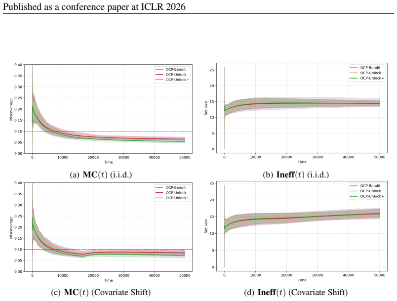
(a)MC(t)(i.i.d.) (b)Ineff(t)(i.i.d.) (c)MC(t)(Non-i.i.d.) (d)Ineff(t)(Non-i.i.d.) Figure 5: Ablation study on ImageNet: Long-run miscoverage MC(t) and inefficiency Ineff(t) as a function of time t∈[T] , under the i.i.d. (top) and non-i.i.d. (bottom) settings. The solid curves denote the average over 50 independent runs, and the shaded regions indicate the...
work page 2026
-
[26]
(a)MC(T)(i.i.d.) (b)MC(T)(Non-i.i.d.) Figure 7: Sensitivity of OCP-Unlock+ to α on ImageNet. Box plots summarize the long-run miscoverage MC(T) across 50 independent runs for α∈ {0.1,0.2,0.3,0.4} under the i.i.d. (left) and non-i.i.d. (right) settings. Each box shows the interquartile range with the median marked inside, while the whiskers indicate the sp...
work page 2026
discussion (0)
Sign in with ORCID, Apple, or X to comment. Anyone can read and Pith papers without signing in.