Predictive Autoscaling for Node.js on Kubernetes: Lower Latency, Right-Sized Capacity
Pith reviewed 2026-05-10 02:02 UTC · model grok-4.3
The pith
A predictive autoscaler for Node.js on Kubernetes forecasts load from cluster-wide invariant metrics to add capacity before overload starts.
A machine-rendered reading of the paper's core claim, the machinery that carries it, and where it could break.
Core claim
The paper establishes that operating on a cluster-wide aggregate metric, which remains approximately invariant under scaling actions, supplies a stable signal for short-term load extrapolation; a three-function metric model plus a five-stage pipeline converts raw, partial, irregularly timed data into this signal, enabling the autoscaler to keep per-instance load near the chosen target throughout both steady ramps and sudden spikes.
What carries the argument
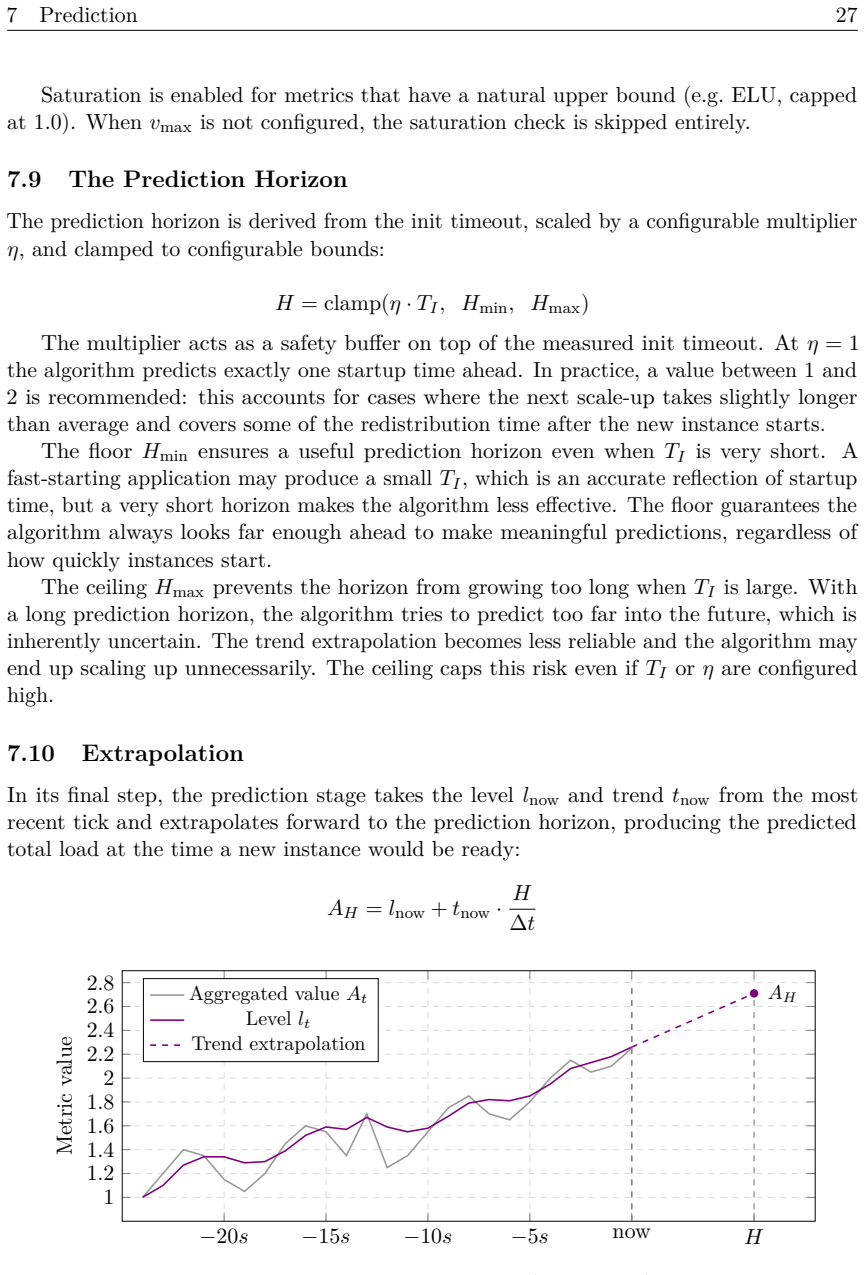
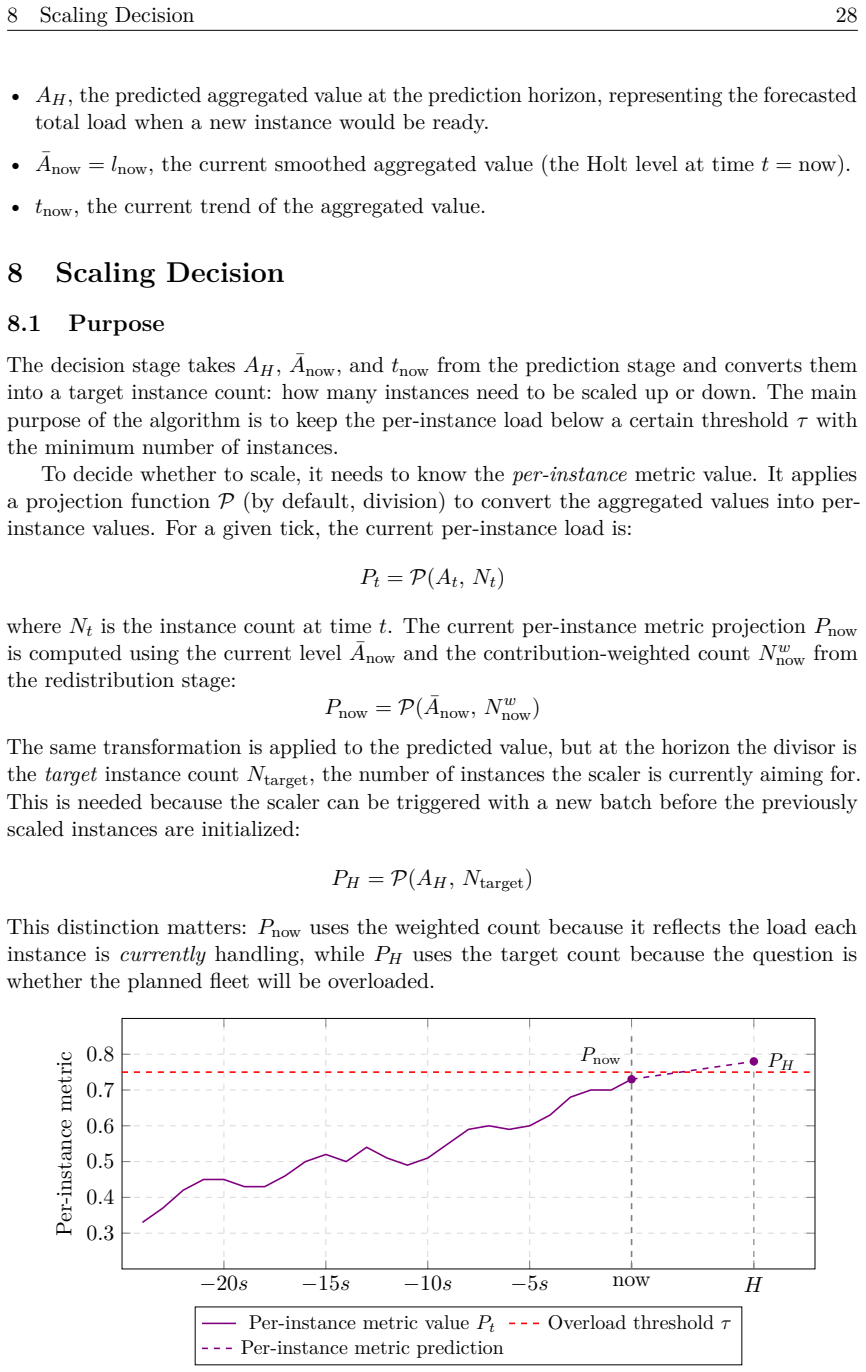
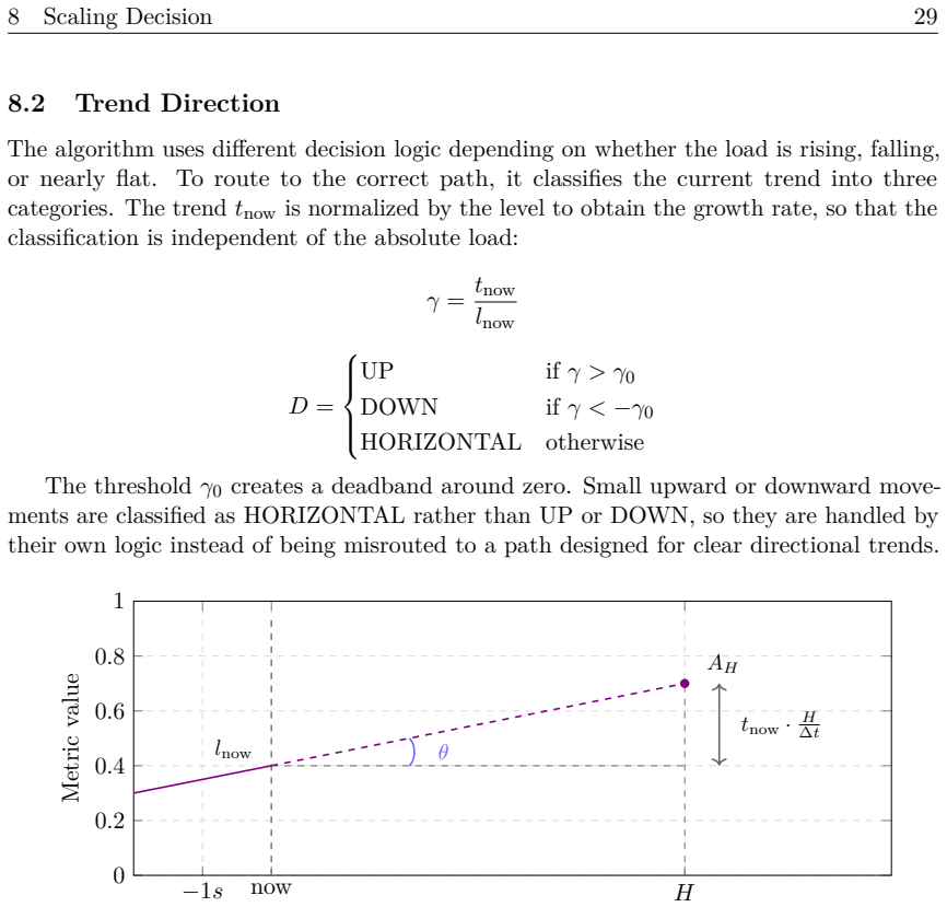
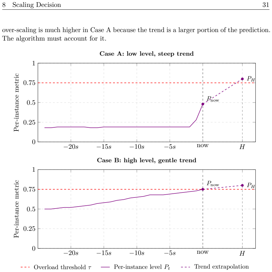
The scaling-invariant cluster-wide aggregate metric, together with a three-function metric model and a five-stage transformation pipeline that produces a clean short-term prediction signal.
If this is right
- Per-instance load stays near the target threshold during both steady ramps and sudden spikes.
- Median latency under steady ramp reaches 26 ms instead of 154 ms with KEDA or 522 ms with HPA.
- Scaling decisions no longer create a feedback loop that corrupts the metrics they rely on.
- Target latency SLOs can be met without lowering thresholds and causing permanent over-provisioning.
Where Pith is reading between the lines
- The same invariant-aggregate idea might apply to other event-driven platforms whose per-instance counters are similarly distorted by scaling.
- Embedding the five-stage pipeline inside KEDA could let operators keep familiar triggers while gaining the predictive step.
- On very large clusters the short-term extrapolation horizon may need recalibration if network or scheduling delays grow.
- Cost models could quantify the reduction in idle capacity once the method is tuned for a given latency target.
Load-bearing premise
A cluster-wide aggregate metric stays approximately the same when new instances are added, giving a reliable signal for predicting load a few minutes ahead even though every per-instance metric changes with each scaling action.
What would settle it
Apply the algorithm to a workload whose cluster-wide aggregate metric shifts markedly after each scaling event; if latency then rises above the reactive baselines instead of staying low, the invariance premise fails.
Figures




read the original abstract
Kubernetes offers two default paths for scaling Node\.js workloads, and both have structural limitations. The Horizontal Pod Autoscaler scales on CPU utilization, which does not directly measure event loop saturation: a Node.js pod can queue requests and miss latency SLOs while CPU reports moderate usage. KEDA extends HPA with richer triggers, including event-loop metrics, but inherits the same reactive control loop, detecting overload only after it has begun. By the time new pods start and absorb traffic, the system may already be degraded. Lowering thresholds shifts the operating point but does not change the dynamic: the scaler still reacts to a value it has already crossed, at the cost of permanent over-provisioning. We propose a predictive scaling algorithm that forecasts where load will be by the time new capacity is ready and scales proactively based on that forecast. Per-instance metrics are corrupted by the scaler's own actions: adding an instance redistributes load and changes every metric, even if external traffic is unchanged. We observe that operating on a cluster-wide aggregate that is approximately invariant under scaling eliminates this feedback loop, producing a stable signal suitable for short-term extrapolation. We define a metric model (a set of three functions that encode how a specific metric relates to scaling) and a five-stage pipeline that transforms raw, irregularly-timed, partial metric data into a clean prediction signal. In benchmarks against HPA and KEDA under steady ramp and sudden spike, the algorithm keeps per-instance load near the target threshold throughout. Under the steady ramp, median latency is 26ms, compared to 154ms for KEDA and 522ms for HPA.
Editorial analysis
A structured set of objections, weighed in public.
Referee Report
Summary. The paper proposes a predictive autoscaling algorithm for Node.js on Kubernetes that forecasts load using a cluster-wide aggregate metric asserted to be approximately invariant under scaling actions, thereby avoiding feedback corruption in per-instance metrics. It introduces a metric model consisting of three functions and a five-stage pipeline to process raw metrics into predictions, enabling proactive scaling. Benchmarks against HPA and KEDA under steady ramp and sudden spike workloads claim that per-instance load stays near the target threshold, with median latency of 26 ms versus 154 ms for KEDA and 522 ms for HPA.
Significance. If the central claims are substantiated, the work could offer a practical improvement for autoscaling latency-sensitive, event-loop-based applications in Kubernetes by enabling right-sized proactive capacity without the over-provisioning or delayed response of reactive methods, addressing a common pain point in cloud deployments of Node.js services.
major comments (2)
- Abstract: The manuscript states specific benchmark outcomes (median latency of 26 ms under steady ramp, load kept near target) but provides no description of the experimental setup, workload generation, cluster configuration, number of runs, statistical significance testing, or implementation details of the five-stage pipeline, rendering the performance claims unverifiable.
- Abstract: The claim that the cluster-wide aggregate metric is 'approximately invariant under scaling' is load-bearing for the predictive mechanism and the assertion that it supplies a stable extrapolation signal, yet the benchmarks report only final latency and load outcomes with no intermediate measurements or quantification of the aggregate value before versus after scale events (holding external arrival rate fixed).
Simulated Author's Rebuttal
We thank the referee for the constructive feedback highlighting areas where the abstract could better support verifiability of our claims. We address each major comment below with targeted revisions that strengthen the manuscript without altering its core contributions.
read point-by-point responses
-
Referee: Abstract: The manuscript states specific benchmark outcomes (median latency of 26 ms under steady ramp, load kept near target) but provides no description of the experimental setup, workload generation, cluster configuration, number of runs, statistical significance testing, or implementation details of the five-stage pipeline, rendering the performance claims unverifiable.
Authors: We agree the abstract's brevity limits inclusion of full experimental details. The complete manuscript details these in Section 4 (cluster: 3-node Kubernetes with 8 vCPU/node; workloads: Locust-generated linear ramp 0-500 req/s and spike to 1000 req/s; 5 runs per condition reporting medians/IQR) and Section 3.3 (five-stage pipeline with pseudocode for ingestion, aggregation, smoothing, forecasting, decision). To improve standalone verifiability, we will revise the abstract to add one sentence summarizing the setup at a high level (e.g., 'evaluated via 5 runs on a 3-node cluster under ramp/spike workloads') while retaining the performance numbers. This provides context without exceeding abstract norms. revision: partial
-
Referee: Abstract: The claim that the cluster-wide aggregate metric is 'approximately invariant under scaling' is load-bearing for the predictive mechanism and the assertion that it supplies a stable extrapolation signal, yet the benchmarks report only final latency and load outcomes with no intermediate measurements or quantification of the aggregate value before versus after scale events (holding external arrival rate fixed).
Authors: The invariance claim is central and is derived in Section 3.1 from the aggregate metric definition (total cluster-wide requests/sec, which is unchanged by pod addition for fixed external arrival rate). The manuscript includes supporting time-series in Figure 5 showing aggregate stability amid per-pod fluctuations during scales. We acknowledge the abstract and main results focus on end-to-end outcomes rather than explicit pre/post quantification. We will add a new table or subsection in the revised manuscript with measurements (e.g., mean absolute change in aggregate value before/after scale events at constant arrival rate) drawn from the existing experimental traces. This directly supplies the requested quantification. revision: yes
Circularity Check
No circularity: claims rest on external benchmarks and an observational assumption, not self-referential derivation
full rationale
The paper defines a metric model with three functions and a five-stage pipeline to generate short-term forecasts from cluster-wide aggregates, then evaluates the resulting autoscaler via direct benchmarks against HPA and KEDA under ramp and spike workloads. No equation or step is shown that reduces a claimed prediction to a fitted parameter by construction, nor does any load-bearing premise rely on a self-citation chain or imported uniqueness theorem. The key assertion that the aggregate metric is approximately invariant under scaling is presented as an empirical observation rather than a derived result; the reported outcomes (median latency 26 ms vs. 154 ms and 522 ms) are measured against independent external controllers, keeping the evaluation self-contained.
Axiom & Free-Parameter Ledger
Forward citations
Cited by 1 Pith paper
-
ADAPT: A Self-Calibrating Proactive Autoscaler for Container Orchestration
ADAPT uses an EWMA estimator for cold-start durations to set a dynamic horizon in an MPC-based proactive autoscaler, achieving under 5% SLA violations with MPC+LSTM across tested workloads versus higher rates for HPA ...
Reference graph
Works this paper leans on
-
[1]
Introduction to Event Loop Utilization in Node.js,
T. Norling, “Introduction to Event Loop Utilization in Node.js,” NodeSource Blog, 2020.https://nodesource.com/blog/event-loop-utilization-nodejs
work page 2020
-
[2]
Kubernetes Authors, “Horizontal Pod Autoscaling,” Kubernetes Documen- tation, 2024. https://kubernetes.io/docs/concepts/workloads/autoscaling/ horizontal-pod-autoscale/
work page 2024
-
[3]
KEDA — Kubernetes Event-driven Autoscaling,
KEDA Contributors, “KEDA — Kubernetes Event-driven Autoscaling,” 2024.https: //keda.sh/docs/ References 46
work page 2024
-
[4]
Knative Authors, “Configuring the Autoscaler,” Knative Documentation, 2024.https: //knative.dev/docs/serving/autoscaling/
work page 2024
-
[5]
Predictive scaling for Amazon EC2 Auto Scaling,
Amazon Web Services, “Predictive scaling for Amazon EC2 Auto Scaling,” AWS Doc- umentation, 2024. https://docs.aws.amazon.com/autoscaling/ec2/userguide/ ec2-auto-scaling-predictive-scaling.html
work page 2024
-
[6]
Forecasting seasonals and trends by exponentially weighted moving aver- ages,
C.C. Holt, “Forecasting seasonals and trends by exponentially weighted moving aver- ages,”International Journal of Forecasting, vol. 20, no. 1, pp. 5–10, 2004. (Original work: ONR Memorandum No. 52, Carnegie Institute of Technology, 1957.)
work page 2004
discussion (0)
Sign in with ORCID, Apple, or X to comment. Anyone can read and Pith papers without signing in.