REVIEW 2 major objections 5 minor 1 cited by
Massive high-redshift galaxies grew most of their stars in short, near-unity-efficiency bursts around z~9-10, unless dust or a top-heavy IMF is allowed for.
Reviewed by Pith at T0; open to challenge. T0 means a machine referee read the full paper against a public rubric. the ladder, T0–T4 →
T0 review · grok-4.5
2026-07-12 15:57 UTC pith:HIZHYPMR
load-bearing objection Clean data-driven SFHs and SFEs from JWST UV LFs; high peaks at z>9 are real predictions of the method, with the usual dust/IMF sensitivity already quantified. the 2 major comments →
How galaxies acquire their stellar mass at high redshift: High star formation efficiencies and the relative roles of dust and initial mass function
The pith
A machine-rendered reading of the paper's core claim, the machinery that carries it, and where it could break.
Core claim
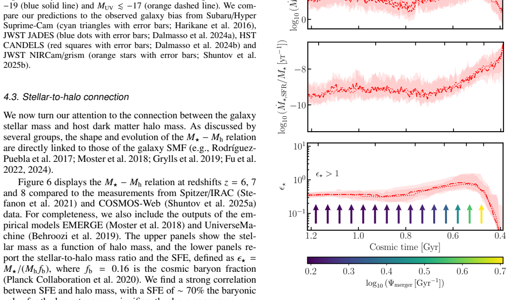
When observed UV luminosity functions at z=5-12 are converted to star-formation rates and abundance-matched to halo accretion rates, massive galaxies are predicted to have assembled most of their stars in a bursty phase around z~9-10 with peak star-formation efficiencies of 0.8-0.9, declining to the familiar 0.2-0.3 only below z~9; dust can push those peaks above unity unless a top-heavy IMF is adopted.
What carries the argument
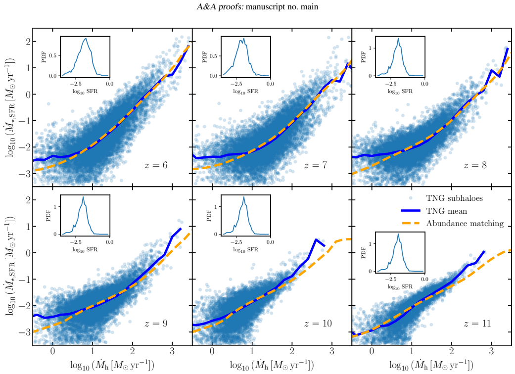
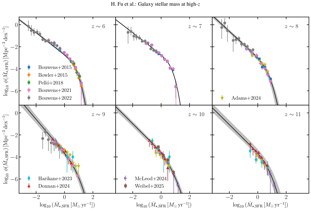
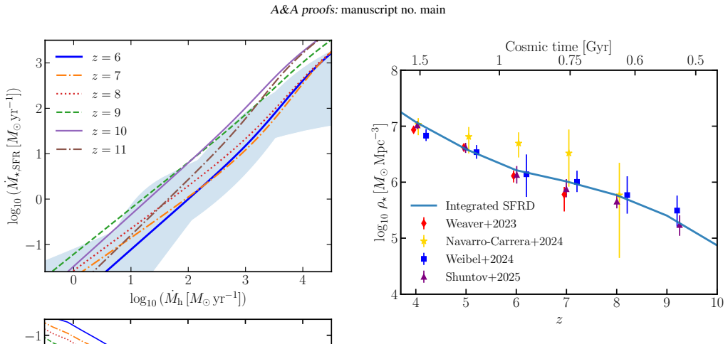
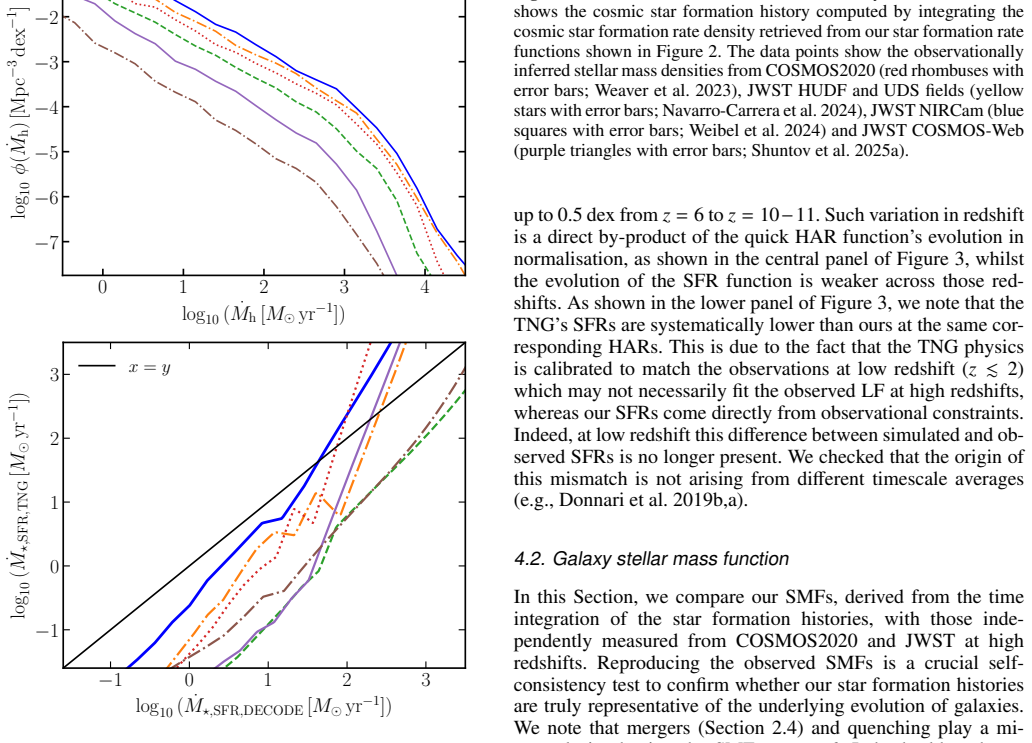
The SFR-halo accretion rate relation recovered by abundance matching the observed UV luminosity function to the theoretical halo accretion-rate distribution (with fixed 0.4 dex scatter); integrating that relation along merger trees yields stellar masses and efficiencies as pure outputs.
Load-bearing premise
That a single monotonic average relation between a galaxy's star-formation rate and its host halo's accretion rate, recovered by abundance matching with fixed scatter, still holds all the way to redshift eleven.
What would settle it
Direct measurements of the infrared luminosity function or of dust-corrected SFRs for a complete sample of massive galaxies at z greater than or equal to 8 that remain well below the UV-inferred rates used here would force the derived efficiencies downward and break the claimed peak near unity.
Editorial analysis
A structured set of objections, weighed in public.
Referee Report
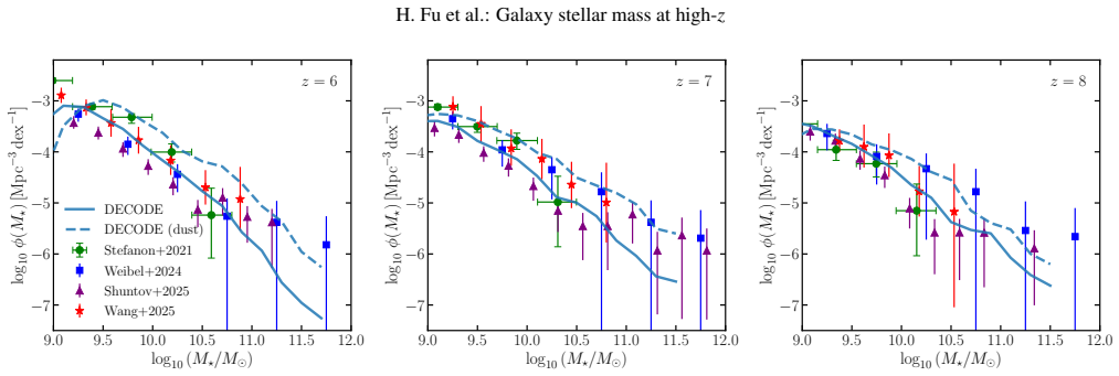
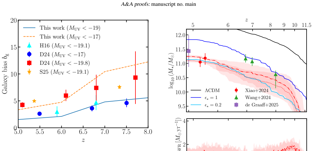
Summary. The paper presents a data-driven semi-empirical model (DECODE) that takes observed UV luminosity functions at z ≃ 5–12 as input, converts them to SFR functions, and abundance-matches them to dark-matter halo accretion-rate distributions (with 0.4 dex scatter) to obtain an SFR–HAR relation. Stellar masses are then built by integrating those SFRs along SatGen merger trees, so that star-formation efficiencies emerge as predictions rather than free parameters. The model reproduces the stellar mass function, large-scale clustering bias, star-forming main sequence and cosmic stellar-mass density. It finds that massive galaxies assemble with a burst at z ∼ 9–10, driving SFEs of 0.8–0.9 that later decline to 0.2–0.3; dust corrections can push SFEs above unity unless a top-heavy IMF is adopted.
Significance. If the central mapping holds, the work supplies a transparent, observationally anchored baseline for high-z SFEs that does not rely on parametric efficiency functions or explicit feedback modelling. The multi-observable consistency checks (SMF, bias, main sequence, stellar-mass density) and the explicit dust/IMF sensitivity tests are genuine strengths; the publicly available DECODE code further aids reproducibility. The result that high SFEs (and a possible variable IMF) are required even in a pure ΛCDM framework is of clear interest to the JWST community and to semi-analytic and simulation groups calibrating early galaxy formation.
major comments (2)
- The load-bearing assumption is the monotonic SFR–HAR relation recovered by abundance matching with fixed 0.4 dex Gaussian scatter (§2.2), validated only against TNG (§3) and then applied to observed UV LFs out to z ∼ 11. The paper already shows that scatter variations of 0.3–0.5 dex shift stellar masses by ≲0.05 dex, and the multi-observable checks provide independent support. Nevertheless, a short quantitative test of how non-monotonicity or redshift-dependent scatter would shift the claimed SFE peaks (0.8–0.9) and the z ∼ 9–10 burst timing would strengthen the central claim without altering the overall architecture.
- Section 4.7 and Appendix C: dust attenuation is applied uniformly across the UV luminosity range, producing SFEs that can exceed unity at z ≳ 7–8. The text notes that the same correction overestimates the faint end of the IR LF (Fig. C.1). A mass- or luminosity-dependent attenuation (or an explicit statement that dust is relevant only for the massive end) is needed to keep the high-SFE claim physically consistent when dust is included.
minor comments (5)
- Equation (1) and surrounding text: the Kennicutt/Madau & Dickinson UV-to-SFR conversion is adopted with only a brief metallicity check; a short table or sentence quantifying the residual systematic for the most massive systems would help readers.
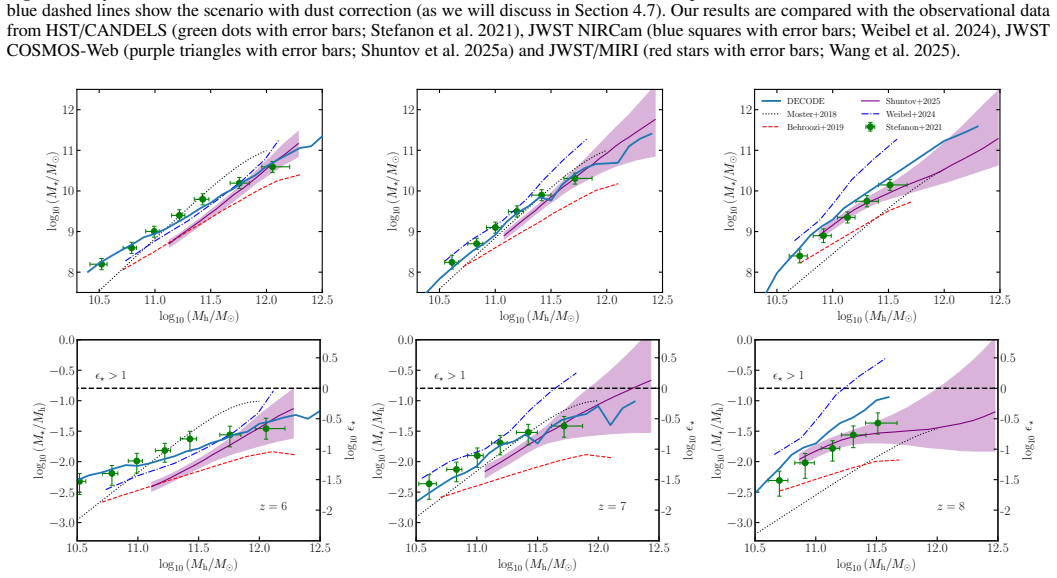
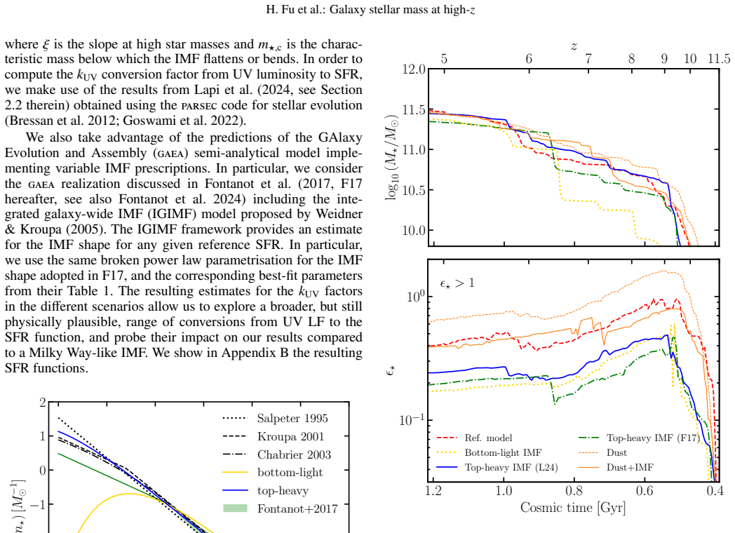
- Figure 6 caption and lower panels: the right-hand SFE axis is defined as ε★ = M★/(Mh fb); a one-line reminder that fb = 0.16 is used would avoid ambiguity.
- Section 2.4: merger timescales are scaled by ∼1.5 at z ≳ 5 relative to Fu et al. (2022); a brief justification or reference for that factor would improve transparency.
- Appendix A, Table A.1: several parameter uncertainties appear without the ‘+’ or ‘−’ signs (e.g., z = 7 row); cosmetic fix only.
- A few typographical slips remain (e.g., ‘decode’ capitalisation, ‘decode’s’, missing spaces around ‘z ∼’).
Circularity Check
No load-bearing circularity: SFEs and SMFs are genuine outputs of UV-LF→SFR–HAR abundance matching plus time integration; only a minor non-forcing self-citation of the authors’ prior DECODE method.
specific steps
-
self citation load bearing
[§2 Methods / DECODE description; also §2.4 mergers]
"we made use, extending it to higher redshifts, of the semi-empirical approach recently devised by our group in two semi-empirical models, decode (Fu et al. 2025a,b) and TopSem (Boco et al. 2023)… These timescales are fitted to reproduce the number densities of surviving satellite subhaloes of the Millennium simulation up to redshift z∼11−12 [referencing Fu et al. 2022]."
The core abundance-matching pipeline and merger-delay prescription are imported from the same authors’ prior DECODE papers rather than re-derived. This is ordinary methodological self-citation and is not load-bearing for the high-z SFE result (the high-z UV LFs and HARs are new inputs), so it raises the score only to 1.
full rationale
The derivation chain is: observed UV LFs → SFR functions (Kennicutt conversion) → abundance matching to theoretical HAR distributions (with fixed 0.4 dex scatter) → SFR–HAR relation → assign SFRs along SatGen progenitor trees → integrate (with recycling) to M⋆ → SFE ≡ M⋆/(Mh fb) and SMF. The SMF, clustering bias, and main sequence are therefore independent consistency checks, not inputs; the paper correctly frames them as such (§4.2–4.4, §4.6). Unlike parametric SFE(Mh,z) models that tune efficiency to match LFs, here SFE is an emergent prediction. Dust and IMF variations are post-hoc sensitivity tests, not free parameters fitted to rescue the high-SFE claim. The only minor circularity-adjacent element is reliance on the authors’ own prior DECODE papers for the low-z method and merger timescales; that is ordinary self-citation of a technique, not a uniqueness theorem or definitional loop that forces the high-z SFE peaks. The TNG scatter and monotonicity assumption are external modelling choices (weakest assumption), not circular reductions. Score 1 reflects that single non-load-bearing self-citation; the central claim does not reduce to its inputs by construction.
Axiom & Free-Parameter Ledger
free parameters (4)
- SFR–HAR scatter =
0.4 dex
- stellar mass recycling fraction R =
0.45
- Saunders SFR-function parameters (ϕ⋆, Ṁ⋆, α, σ) at each z =
see Table A.1
- Larson IMF characteristic mass / high-mass slope for toy models =
m⋆,c=0.1 M⊙; ξ=−1.5
axioms (5)
- domain assumption Mean galaxy SFR is a monotonic function of host-halo accretion rate that can be recovered by abundance matching
- domain assumption Planck 2020 ΛCDM cosmology and Tinker halo mass function / bias
- domain assumption UV luminosity converts to SFR via Kennicutt/Madau factor (kUV=2.5×10⁻¹⁰) for a Chabrier IMF, with only mild metallicity corrections
- domain assumption Satellite galaxies follow the same M⋆–Mh relation as centrals at infall and merge on delayed timescales calibrated to Millennium
- domain assumption Dust attenuation can be described by Charlot & Fall, Calzetti or Salim curves with literature parameters
Cite this review
Pith. "Pith review of How galaxies acquire their stellar mass at high redshift: High star formation efficiencies and the relative roles of dust and initial mass function." pith.science (2026). https://pith.science/paper/HIZHYPMR
@misc{pith2026260526209,
  author       = {Pith},
  title        = {Pith review of: How galaxies acquire their stellar mass at high redshift: High star formation efficiencies and the relative roles of dust and initial mass function},
  year         = {2026},
  howpublished = {\url{https://pith.science/paper/HIZHYPMR}},
  note         = {Machine review of arXiv:2605.26209}
}
read the original abstract
JWST has measured an unprecedented abundance of galaxies above $z\gtrsim 4-5$, whose formation and evolution are still difficult to reconcile within traditional galaxy evolution models in a $\Lambda$CDM framework. Here, we present a study on the star formation histories of these high-redshift galaxies between $z\simeq5-12$ via a data-driven semi-empirical model that uses the observed UV LFs as input to retrieve SFRs, naturally bypassing any uncertain modelling of cooling, feedback and/or stochastic processes. Galaxy stellar masses are progressively built in time by integrating their SFRs assigned along their progenitor haloes via the SFR-halo accretion rate relation, derived from abundance matching between the input observed UV LFs with the dark matter halo accretion rate distributions at each redshift. This makes the SFEs a full prediction of the model rather than a tuned input, serving as a natural baseline to test burstiness, dust attenuation, or IMF variations. Our approach naturally reproduces the total stellar mass function, the large-scale clustering, and the star-forming main sequence. We find that massive galaxies grew their stellar mass with a bursty star formation at $z\sim9-10$, broadly in agreement with the star formation histories inferred from spectral energy distribution fitting, with the SFE reaching high peaks of $0.8-0.9$ at $z>9$ and lowering to standard values of $0.2-0.3$ below $z\lesssim9$. We find that the presence of dust could enhance the predicted SFRs at $z\lesssim8$, better reproducing the observed SFRs of massive dusty galaxies, and increase the SFEs to values close to or even above unity at $z \gtrsim 8$. Finally, switching to top-heavy IMFs reduces the SFEs by a factor of $2-3$, highlighting the need for a variable IMF as an inevitable ingredient in the evolution of galaxies at high redshifts to avoid unphysical SFEs, especially in the presence of dust.
Figures
Forward citations
Cited by 1 Pith paper
-
Do we understand the star formation history of the universe?
Star formation rates required by the evolving stellar mass function yield a main sequence that agrees with JWST spectroscopy and theory but differs from prior concordance relations.
Reference graph
Works this paper leans on
-
[1]
J., Conselice, C
Adams, N. J., Conselice, C. J., Austin, D., et al. 2024, ApJ, 965, 169
2024
-
[2]
B., Casey, C
Akins, H. B., Casey, C. M., Lambrides, E., et al. 2025, ApJ, 991, 37
2025
-
[3]
Algera, H. S. B., Inami, H., Oesch, P. A., et al. 2023, MNRAS, 518, 6142
2023
-
[4]
2015, ApJ, 810, 74
Aversa, R., Lapi, A., de Zotti, G., Shankar, F., & Danese, L. 2015, ApJ, 810, 74
2015
-
[5]
M., Valentino, F., Lagos, C
Baker, W. M., Valentino, F., Lagos, C. d. P., et al. 2025, A&A, 702, A270
2025
-
[6]
H., Hearin, A
Behroozi, P., Wechsler, R. H., Hearin, A. P., & Conroy, C. 2019, MNRAS, 488, 3143
2019
-
[7]
R., Drory, N., & Sheth, R
Bernardi, M., Domínguez Sánchez, H., Brownstein, J. R., Drory, N., & Sheth, R. K. 2019, MNRAS, 489, 5633
2019
-
[8]
B., et al
Bernardi, M., Shankar, F., Hyde, J. B., et al. 2010, MNRAS, 404, 2087
2010
-
[9]
& Fritze-v
Bicker, J. & Fritze-v. Alvensleben, U. 2005, A&A, 443, L19
2005
-
[10]
2023, ApJ, 954, 97
Boco, L., Lapi, A., Shankar, F., et al. 2023, ApJ, 954, 97
2023
-
[11]
2025, ApJ, 984, 117
Bosi, M., Lapi, A., Boco, L., et al. 2025, ApJ, 984, 117
2025
-
[12]
2015, A&A, 575, A56
Bournaud, F., Daddi, E., Weiß, A., et al. 2015, A&A, 575, A56
2015
-
[13]
2023, MNRAS, 523, 1009
Bouwens, R., Illingworth, G., Oesch, P., et al. 2023, MNRAS, 523, 1009
2023
-
[14]
J., Illingworth, G., Ellis, R
Bouwens, R. J., Illingworth, G., Ellis, R. S., Oesch, P., & Stefanon, M. 2022, ApJ, 940, 55
2022
-
[15]
J., Illingworth, G
Bouwens, R. J., Illingworth, G. D., Oesch, P. A., et al. 2015, ApJ, 803, 34
2015
-
[16]
J., Oesch, P
Bouwens, R. J., Oesch, P. A., Stefanon, M., et al. 2021, AJ, 162, 47
2021
-
[17]
Bowler, R. A. A., Dunlop, J. S., McLure, R. J., et al. 2015, MNRAS, 452, 1817
2015
-
[18]
2023, Nature Astronomy, 7, 731
Boylan-Kolchin, M. 2023, Nature Astronomy, 7, 731
2023
-
[19]
2012, MNRAS, 427, 127
Bressan, A., Marigo, P., Girardi, L., et al. 2012, MNRAS, 427, 127
2012
-
[20]
Buchan, S. & Shankar, F. 2016, MNRAS, 462, 2001 Calabrò, A., Pentericci, L., Llerena, M., et al. 2026, arXiv e-prints, arXiv:2602.18068
arXiv 2016
-
[21]
C., et al
Calzetti, D., Armus, L., Bohlin, R. C., et al. 2000, ApJ, 533, 682
2000
-
[22]
2006, MNRAS, 366, 1126
Cappellari, M., Bacon, R., Bureau, M., et al. 2006, MNRAS, 366, 1126
2006
-
[23]
C., Begley, R., McLeod, D
Carnall, A. C., Begley, R., McLeod, D. J., et al. 2023, MNRAS, 518, L45
2023
-
[24]
C., Cullen, F., McLure, R
Carnall, A. C., Cullen, F., McLure, R. J., et al. 2024, MNRAS, 534, 325
2024
-
[25]
2003, PASP, 115, 763
Chabrier, G. 2003, PASP, 115, 763
2003
-
[26]
& Fall, S
Charlot, S. & Fall, S. M. 2000, ApJ, 539, 718
2000
-
[27]
E., Sanders, R
Clarke, L., Shapley, A. E., Sanders, R. L., et al. 2024, ApJ, 977, 133
2024
-
[28]
2026, Journal of High Energy Astro- physics, 53, 100626
Comini, L., Vagnozzi, S., & Loeb, A. 2026, Journal of High Energy Astro- physics, 53, 100626
2026
-
[29]
& van Dokkum, P
Conroy, C. & van Dokkum, P. G. 2012, ApJ, 760, 71
2012
-
[30]
J., McLure, R
Cullen, F., McLeod, D. J., McLure, R. J., et al. 2024, MNRAS, 531, 997
2024
-
[31]
2023, MNRAS, 518, 425
Curti, M., D’Eugenio, F., Carniani, S., et al. 2023, MNRAS, 518, 425
2023
-
[32]
2023, Nature Astronomy, 7, 622
Curtis-Lake, E., Carniani, S., Cameron, A., et al. 2023, Nature Astronomy, 7, 622
2023
-
[33]
2024b, MNRAS, 528, 898 Davé, R., Anglés-Alcázar, D., Narayanan, D., et al
Dalmasso, N., Trenti, M., & Leethochawalit, N. 2024b, MNRAS, 528, 898 Davé, R., Anglés-Alcázar, D., Narayanan, D., et al. 2019, MNRAS, 486, 2827 de Graaff, A., Setton, D. J., Brammer, G., et al. 2025, Nature Astronomy, 9, 280
2019
-
[34]
& Birnboim, Y
Dekel, A. & Birnboim, Y . 2006, MNRAS, 368, 2
2006
-
[35]
2009, Nature, 457, 451
Dekel, A., Birnboim, Y ., Engel, G., et al. 2009, Nature, 457, 451
2009
-
[36]
2025, MNRAS, 544, 160
Dekel, A., Mandelker, N., Li, Z., et al. 2025, MNRAS, 544, 160
2025
-
[37]
C., Birnboim, Y ., Mandelker, N., & Li, Z
Dekel, A., Sarkar, K. C., Birnboim, Y ., Mandelker, N., & Li, Z. 2023, MNRAS, 523, 3201
2023
-
[38]
T., McLure, R
Donnan, C. T., McLure, R. J., Dunlop, J. S., et al. 2024, MNRAS, 533, 3222
2024
-
[39]
2025, ApJ, 982, L12
Dou, J., Peng, Y ., Gu, Q., et al. 2025, ApJ, 982, L12
2025
-
[40]
2023, MNRAS, 519, 2199 Enríquez-Vargas, M., Rodríguez-Puebla, A., Manuwal, A., et al
Eisert, L., Pillepich, A., Nelson, D., et al. 2023, MNRAS, 519, 2199 Enríquez-Vargas, M., Rodríguez-Puebla, A., Manuwal, A., et al. 2026, arXiv e- prints, arXiv:2605.08353 Euclid Collaboration, Mellier, Y ., Abdurro’uf, et al. 2025, A&A, 697, A1
Pith/arXiv arXiv 2023
-
[41]
2026, ApJ, 998, 178
Fakhry, S., Shiravand, M., & Del Popolo, A. 2026, ApJ, 998, 178
2026
-
[42]
2024, A&A, 684, A207
Ferrara, A. 2024, A&A, 684, A207
2024
-
[43]
2023, MNRAS, 522, 3986
Ferrara, A., Pallottini, A., & Dayal, P. 2023, MNRAS, 522, 3986
2023
-
[44]
2022, MNRAS, 512, 58
Ferrara, A., Sommovigo, L., Dayal, P., et al. 2022, MNRAS, 512, 58
2022
-
[45]
L., Bagley, M
Finkelstein, S. L., Bagley, M. B., Ferguson, H. C., et al. 2023, ApJ, 946, L13
2023
-
[46]
L., Leung, G
Finkelstein, S. L., Leung, G. C. K., Bagley, M. B., et al. 2024, ApJ, 969, L2
2024
-
[47]
Fitzpatrick, E. L. & Massa, D. 1986, ApJ, 307, 286
1986
-
[48]
2017, MNRAS, 464, 3812
Fontanot, F., De Lucia, G., Hirschmann, M., et al. 2017, MNRAS, 464, 3812
2017
-
[49]
2026, arXiv e-prints, arXiv:2603.22405
Fontanot, F., De Lucia, G., Xie, L., et al. 2026, arXiv e-prints, arXiv:2603.22405
arXiv 2026
-
[50]
2024, A&A, 686, A302
Fontanot, F., La Barbera, F., De Lucia, G., et al. 2024, A&A, 686, A302
2024
-
[51]
2022, MNRAS, 516, 3206
Fu, H., Shankar, F., Ayromlou, M., et al. 2022, MNRAS, 516, 3206
2022
-
[52]
2024, MNRAS, 532, 177 Article number, page 13 of 16 A&A proofs:manuscript no
Fu, H., Shankar, F., Ayromlou, M., et al. 2024, MNRAS, 532, 177 Article number, page 13 of 16 A&A proofs:manuscript no. main
2024
-
[53]
Gelli, V ., Mason, C., & Hayward, C. C. 2024, ApJ, 975, 192
2024
-
[54]
2000, A&AS, 141, 371
Girardi, L., Bressan, A., Bertelli, G., & Chiosi, C. 2000, A&AS, 141, 371
2000
-
[55]
2024, Nature, 628, 277
Glazebrook, K., Nanayakkara, T., Schreiber, C., et al. 2024, Nature, 628, 277
2024
-
[56]
2022, A&A, 663, A1
Goswami, S., Silva, L., Bressan, A., et al. 2022, A&A, 663, A1
2022
-
[57]
2020, A&A, 643, A8
Gruppioni, C., Béthermin, M., Loiacono, F., et al. 2020, A&A, 643, A8
2020
-
[58]
J., Shankar, F., Leja, J., et al
Grylls, P. J., Shankar, F., Leja, J., et al. 2020, MNRAS, 491, 634
2020
-
[59]
J., Shankar, F., Zanisi, L., & Bernardi, M
Grylls, P. J., Shankar, F., Zanisi, L., & Bernardi, M. 2019, MNRAS, 483, 2506
2019
-
[60]
K., Ellis, R
Harikane, Y ., Inoue, A. K., Ellis, R. S., et al. 2025, ApJ, 980, 138
2025
-
[61]
2023, ApJS, 265, 5
Harikane, Y ., Ouchi, M., Oguri, M., et al. 2023, ApJS, 265, 5
2023
-
[62]
2016, ApJ, 821, 123
Harikane, Y ., Ouchi, M., Ono, Y ., et al. 2016, ApJ, 821, 123
2016
-
[63]
Hopkins, A. M. 2018, PASA, 35, e039
2018
-
[64]
F., Quataert, E., & Murray, N
Hopkins, P. F., Quataert, E., & Murray, N. 2011, MNRAS, 417, 950
2011
-
[65]
K., Li, W., & Ho, L
Inayoshi, K., Harikane, Y ., Inoue, A. K., Li, W., & Ho, L. C. 2022, ApJ, 938, L10 Ivezi´c, Ž., Kahn, S. M., Tyson, J. A., et al. 2019, ApJ, 873, 111
2022
-
[66]
K., Carnall, A
Jespersen, C. K., Carnall, A. C., & Lovell, C. C. 2025, ApJ, 988, L19
2025
-
[67]
2021, MNRAS, 502, 621 Juodžbalis, I., Maiolino, R., Baker, W
Jiang, F., Dekel, A., Freundlich, J., et al. 2021, MNRAS, 502, 621 Juodžbalis, I., Maiolino, R., Baker, W. M., et al. 2026, MNRAS, 546, stag086
2021
-
[68]
2026, ApJ, 996, 103
Kar, A., Alam, S., & Silk, J. 2026, ApJ, 996, 103
2026
-
[69]
Kennicutt, Jr., R. C. 1998, ARA&A, 36, 189
1998
-
[70]
2001, MNRAS, 322, 231 La Barbera, F., Vazdekis, A., Ferreras, I., et al
Kroupa, P. 2001, MNRAS, 322, 231 La Barbera, F., Vazdekis, A., Ferreras, I., et al. 2016, MNRAS, 457, 1468 Labbé, I., van Dokkum, P., Nelson, E., et al. 2023, Nature, 616, 266
2001
-
[71]
2026, in Encyclopedia of Astrophysics, V olume 4, V ol
Lapi, A., Boco, L., & Shankar, F. 2026, in Encyclopedia of Astrophysics, V olume 4, V ol. 4, 554–575
2026
-
[72]
2024, Universe, 10, 141
Lapi, A., Gandolfi, G., Boco, L., et al. 2024, Universe, 10, 141
2024
-
[73]
Larson, R. B. 1998, MNRAS, 301, 569
1998
-
[74]
S., Ting, Y .-S., et al
Leja, J., Speagle, J. S., Ting, Y .-S., et al. 2022, ApJ, 936, 165
2022
-
[75]
C., Harrison, I., Harikane, Y ., Tacchella, S., & Wilkins, S
Lovell, C. C., Harrison, I., Harikane, Y ., Tacchella, S., & Wilkins, S. M. 2023, MNRAS, 518, 2511
2023
-
[76]
2024, MNRAS, 530, 4474
Lu, S., Zhu, K., Cappellari, M., et al. 2024, MNRAS, 530, 4474
2024
-
[77]
& Dickinson, M
Madau, P. & Dickinson, M. 2014, ARA&A, 52, 415
2014
-
[78]
2018, MNRAS, 480, 5113
Marinacci, F., V ogelsberger, M., Pakmor, R., et al. 2018, MNRAS, 480, 5113
2018
-
[79]
2022, MNRAS, 510, 5639
Marsden, C., Shankar, F., Bernardi, M., et al. 2022, MNRAS, 510, 5639
2022
-
[80]
A., Trenti, M., & Treu, T
Mason, C. A., Trenti, M., & Treu, T. 2023, MNRAS, 521, 497
2023
discussion (0)
Sign in with ORCID, Apple, or X to comment. Anyone can read and Pith papers without signing in.