REVIEW 3 major objections 5 minor 1 cited by
A pilot-fitted deterministic denominator removes mean-shift bias from tamed SGLD while matching the expensive growth-score envelope.
Reviewed by Pith at T0; open to challenge. T0 means a machine referee read the full paper against a public rubric. the ladder, T0–T4 →
T0 review · grok-4.5
2026-07-12 14:25 UTC pith:TKAWFA4O
load-bearing objection Solid methods paper: pilot-proxy deterministic denominators fix a real mean-shift bias in tamed SGLD, with careful residual bookkeeping and supportive quartic experiments. the 3 major comments →
Deterministic Denominator Design for Localized Tamed Stochastic Gradient Langevin Dynamics
The pith
A machine-rendered reading of the paper's core claim, the machinery that carries it, and where it could break.
Core claim
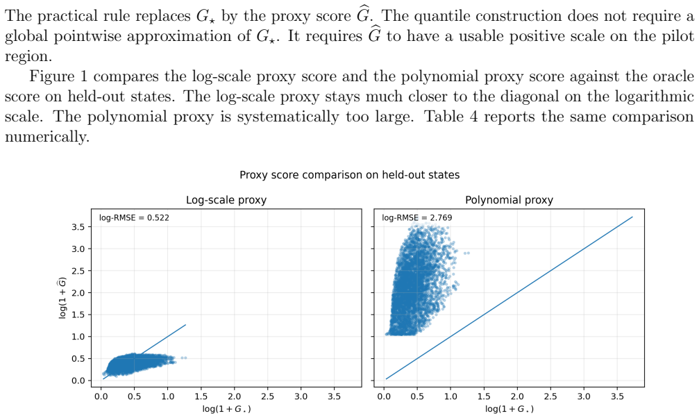
A state-dependent denominator fixed before the current stochastic-gradient draw eliminates the mean-shift bias of random-denominator taming. Building that denominator from a pilot-fitted log-scale proxy of the growth score G⋆ and from empirical pilot quantiles yields a local proxy-quantile envelope whose finite-chain observables stay close to the exact G⋆-envelope while improving on random-denominator tamed SGLD at comparable production cost, with proxy and threshold errors controlled into stationary observable error.
What carries the argument
The proxy-quantile localized envelope: a shifted-log least-squares proxy bG of G⋆ is combined with pilot quantiles of bG to form Aloc = (bG − R̂)+^θ + (bG − Ŝ)+; the production denominator is then Dη,loc = 1 + η^α Aloc. Cone comparison on the pilot region turns log-scale accuracy into level-set and positive-part sandwiches, which transfer into envelope, modified-drift, and stationary residual bounds.
Load-bearing premise
The pilot run and the chosen features must capture the growth-score geometry well enough that the fitted proxy stays multiplicatively close to the true growth score on the region the chain actually visits.
What would settle it
On the same high-dimensional quartic-regression instances, replace the pilot-fitted log-radial proxy by a deliberately biased or under-covered feature map and check whether the reported order-of-magnitude gap reduction relative to random-denominator and global-hard baselines disappears while the G⋆-envelope reference remains unchanged.
Editorial analysis
A structured set of objections, weighed in public.
Referee Report
Summary. The paper designs practical deterministic denominators for localized tamed SGLD. It starts from the observation that a denominator depending on the current stochastic-gradient draw can bias the conditional mean even for an unbiased oracle, and removes that coupling by fixing a state-dependent denominator before the draw. The growth score G★(x)=∥b(x)∥/(1+∥x∥) is taken as the ideal deterministic growth indicator; a shifted-log proxy is fitted from a short pilot run, pilot quantiles set soft/hard activation thresholds, and the resulting local proxy-quantile envelope is used as the production denominator. A separate norm-polynomial tail floor is introduced only when one wants the global effective-linearity input of the companion deterministic-envelope Lyapunov theory. The analysis transfers log-scale proxy and quantile errors into envelope, modified-drift, and stationary-observable residuals (conditional on local cone comparison and the companion Poisson/Lyapunov framework). Experiments on quartic regression show the local proxy-quantile denominator tracks the G★-envelope closely, improves over random-denominator and global-hard baselines at comparable production cost, and activates the tail floor only sparsely.
Significance. If the claims hold, the paper supplies a concrete, low-cost design rule for deterministic denominators in tamed SGLD: pilot-fit a log-scale proxy of G★, calibrate localized thresholds by quantiles, and optionally add a cheap polynomial tail floor for global Lyapunov certification. That is a useful engineering contribution for nonconvex sampling with superlinear drifts, where random denominators introduce a mean-shift channel and full-gradient growth scores are expensive. Strengths include a careful comparison-and-transfer analysis (cone comparison, level-set/positive-part sandwiches, Markov quantile stability, envelope-to-drift residuals, and a bookkeeping stationary residual), an explicit local-vs-global distinction between Dη,loc and Dη,final, sandwich diagnostics (Tables 3–4), and production-cost evidence that the proxy stays near the random-denominator regime (Table 10). The work is tightly coupled to the companion framework [24] and is validated mainly on quartic regression, so its significance is as a design-and-transfer paper rather than a standalone convergence theory.
major comments (3)
- Assumption 1 (§3.4) is load-bearing for the local proxy-quantile claim: cone comparison, level-set/positive-part sandwiches (Props. 3.2–3.3), quantile transfer (Prop. 3.8, Lem. 3.9), envelope residual (Cor. 4.2), and the pilot-region part of the stationary residual (Prop. 4.4 / (4.14)) all require local L∞ control of the log-scale proxy on the visited set. The default log-radial feature is only shown to be adequate for the reported quartic targets (Tables 3–4, 5–8). The manuscript should state more sharply that the main experimental claims are conditional on this local calibration holding where the chain visits, and should either (i) report a simple post-pilot diagnostic of ∥bh−L★∥L∞ or violation mass on held-out pilot states as a required check, or (ii) add at least one non-radial / anisotropic risk where the default feature is expected to be stressed, so that the scope of the design is
- The stationary-error transfer (Prop. 4.4, display (4.14)) and the global stability statement for Dη,final (Prop. 3.11) both invoke the companion deterministic-envelope Lyapunov/Poisson theory [24, Prop. 4.6, Thm. 4.4, Thm. 7.5, Prop. 7.2] rather than re-deriving the Poisson bridge or moment bounds. That is legitimate as a transfer paper, but the abstract and introduction currently read as if the stationary-observable control is self-contained. The claims should be phrased as residual bookkeeping under the companion hypotheses, and the manuscript should list explicitly which companion assumptions are inherited (especially for the stochastic-gradient case and the polynomial upper growth of Dη,loc).
- Empirical support is concentrated on one risk family (quartic regression with λ∥w∥²/2). Tables 5–8 and the d=50 sweep show a clear advantage over random-denominator and global-hard baselines and proximity to the G★-envelope, but they do not yet establish that the same pilot-proxy design works for other superlinear nonconvex targets (e.g., multimodal or anisotropic drifts). A second target, even at modest dimension, would substantially strengthen the central experimental claim that the local proxy-quantile denominator is a practical general design rather than a quartic-specific fit.
minor comments (5)
- Notation for the stochastic-gradient oracle is slightly inconsistent: bgm appears both as a gradient-style oracle and, after a sign flip, as a drift oracle (§2.1). A single convention would reduce confusion when reading the update (5.2).
- Table 1 lists Dη,loc and Dη,final, but the experimental protocol (§5) mostly writes Dη,α,qR,qS,θ. Aligning the experimental notation with the design summary in §3.8 would help.
- The default quantile levels qR=0.70, qS=0.99 and θ=1/2 are stated as a fixed convention (§3.6) with little sensitivity discussion. A short note or appendix table on mild variation of (qR,qS,θ) would make the design less opaque.
- In Experiment 5.1 the diagnostic δ is not used by the algorithm; that is correctly stated, but the text could more clearly separate “algorithm parameters” from “diagnostic tolerances” to avoid readers treating δ as a free design knob.
- Minor typography: “Key W ords” in the front matter; a few long displayed inequalities (e.g., (4.14)) would benefit from tighter line breaks for readability.
Circularity Check
No derivation-by-construction circularity; only load-bearing self-citation of the authors' companion Lyapunov/Poisson framework for stability and stationary transfer, while proxy design and experiments remain independent.
specific steps
-
self citation load bearing
[§3.7 Prop. 3.11; §4.3 Prop. 4.4 / (4.6)–(4.9)]
"Then Dη,final is state-deterministic and satisfies the global effective-linearity input (3.14). ... Then the exact-gradient kernel with denominator Dη,final satisfies the Lyapunov drift estimate of [24, Proposition 4.6], admits invariant measures, and has the uniform moment bounds of [24, Theorem 4.4]. ... We use the stationary Poisson-bridge estimate from the companion deterministic-envelope paper, namely [24, Theorem 7.5]. ... Applying [24, Theorem 7.5] gives |πfinalη(H)−π(H)| ≤ ..."
Global stability of the tail-corrected denominator and the stationary observable-error transfer are not proved in this paper; they are imported wholesale from the same authors' companion arXiv:2606.05242. The present residual bookkeeping (proxy-transfer vs G⋆-envelope vs tail floor) is new organization, but the load-bearing Lyapunov drift, invariant-measure existence, moment bounds, and Poisson-bridge inequality rest only on that overlapping-author citation. This is self-citation load-bearing for the theoretical half of the strongest claim, not a by-construction collapse of the proxy fit or the experiments.
full rationale
The paper's core construction is open calibration, not a disguised prediction: a log-scale proxy is least-squares fitted to pilot G⋆ labels, pilot quantiles set thresholds, and theory then bounds the residual under cone comparison (Assumption 1, Props. 3.2–3.4, 3.8, Cor. 4.2). That is definitional design, not claiming that the fit independently predicts the fitted quantity. The elementary mean-identity for a state-fixed denominator is self-contained. Experimental claims (Tables 5–8, 10) compare production-chain observables against exact-gradient, G⋆-envelope, random-denominator, and global-hard baselines at fixed protocol; those gaps are not forced by the pilot fit. The only circularity-adjacent pattern is self-citation of the same authors' companion [24] for the global Lyapunov input (Prop. 3.11) and the Poisson-bridge stationary residual transfer (Prop. 4.4 invoking [24, Thm. 7.5]). That makes the theoretical stability/transfer claims conditional on an overlapping-author framework rather than re-derived here, but it does not reduce the proxy-design or experimental claims to their inputs by construction. Score 2: one load-bearing self-citation chain that is not uniqueness-forcing and does not collapse the main empirical contribution.
Axiom & Free-Parameter Ledger
free parameters (6)
- qR, qS (pilot quantile levels) =
0.70, 0.99
- θ (soft-transition exponent) =
1/2
- τ (log-shift floor) =
max(1e-6, 0.01*median pilot G⋆)
- bω (proxy regression coefficients) =
pilot least-squares solution
- α, η (taming multiplier and stepsize)
- κtail, qlin, qtail, ρlin (tail-floor parameters) =
κtail=2; qlin=0.95; qtail=0.995; ρlin=1
axioms (6)
- domain assumption Polynomial local Lipschitz and dissipative drift assumptions of the companion Langevin setting (§2.1).
- domain assumption Unbiased stochastic-gradient oracle with conditional mean zero noise (§2.1).
- ad hoc to paper Assumption 1: local L∞ approximation bias and L2→L∞ norm control of the feature class on the pilot region (§3.4).
- domain assumption Assumptions 2–3: nondegenerate quantile crossing and Markov pilot concentration at quantile endpoints (§3.5).
- domain assumption Companion deterministic-envelope Lyapunov, invariant-measure, and Poisson-bridge results [24, Prop 4.6, Thm 4.4, Thm 7.5, Prop 7.2].
- ad hoc to paper Polynomial-tail domination G⋆(x) ≤ Ctail Ptail(x) on all of R^d (3.19) when certifying the final denominator.
invented entities (3)
-
Growth score G⋆(x)=||b(x)||/(1+||x||) as deterministic growth indicator
independent evidence
-
Proxy-quantile localized envelope Aloc / Dη,loc
independent evidence
-
Norm-polynomial tail floor Dη,tail / Dη,final
independent evidence
read the original abstract
If the denominator in a tamed stochastic gradient Langevin update uses the current stochastic-gradient draw, the conditional mean can be biased even when the stochastic-gradient oracle is unbiased. A state-dependent denominator fixed before that draw removes this coupling. We build practical deterministic denominators from a short pilot run. A log-scale proxy is fitted to the growth score $G_\star(x)=\|b(x)\|/(1+\|x\|)$, and empirical pilot quantiles set the activation thresholds of a local proxy-quantile envelope. The reported proxy-quantile experiments use this local denominator. Separately, we describe a final denominator with a norm-polynomial tail-floor correction that can be used when one wants to certify the global effective-linearity input required by the companion deterministic-envelope Lyapunov theory. We show how proxy and threshold errors enter denominator errors and the resulting stationary observable errors. In the reported experiments, the local proxy-quantile denominator improves over random-denominator tamed SGLD at comparable production cost. It also gives observable behavior close to the $G_\star$-envelope benchmark, without the full-gradient growth-score evaluations required by that benchmark.
Figures
Forward citations
Cited by 1 Pith paper
-
RELTA-SGLD: Relative-Growth Localized Taming for Nonconvex Stochastic-Gradient Langevin Learning
A relative-growth, threshold-localized taming denominator for SGLD achieves O(λ) stationary W1 and (in the potential case) W2 accuracy for nonconvex superlinear stochastic-gradient oracles.
Reference graph
Works this paper leans on
-
[1]
Welling and Y
M. Welling and Y. W. Teh. Bayesian learning via stochastic gradient Langevin dynamics. Proceedings of the 28th International Conference on Machine Learning (ICML), pp. 681–688, 32 2011
2011
-
[2]
S. J. Vollmer, K. C. Zygalakis, and Y. W. Teh. Exploration of the (non-)asymptotic bias and variance of stochastic gradient Langevin dynamics.Journal of Machine Learning Research, 17(159):1–48, 2016
2016
-
[3]
T. Chen, E. B. Fox, and C. Guestrin. Stochastic gradient Hamiltonian Monte Carlo. Proceedings of the 31st International Conference on Machine Learning, PMLR 32(2):1683–1691, 2014
2014
-
[4]
Y.-A. Ma, T. Chen, and E. B. Fox. A complete recipe for stochastic gradient MCMC. Advances in Neural Information Processing Systems, 28, 2015
2015
-
[5]
Brosse, A
N. Brosse, A. Durmus, and E. Moulines. The promises and pitfalls of stochastic gradient Langevin dynamics.Advances in Neural Information Processing Systems, 31, 2018
2018
-
[6]
K. A. Dubey, S. J. Reddi, S. A. Williamson, B. P´ oczos, A. J. Smola, and E. P. Xing. Variance reduction in stochastic gradient Langevin dynamics.Advances in Neural Information Processing Systems, 29, 2016
2016
-
[7]
C. Li, C. Chen, D. Carlson, and L. Carin. Preconditioned stochastic gradient Langevin dynamics for deep neural networks.Proceedings of the AAAI Conference on Artificial Intelligence, 30(1), 2016
2016
-
[8]
Raginsky, A
M. Raginsky, A. Rakhlin, and M. Telgarsky. Non-convex learning via stochastic gradient Langevin dynamics: a nonasymptotic analysis.Proceedings of the 2017 Conference on Learning Theory, PMLR 65:1674–1703, 2017
2017
-
[9]
D. Zou, P. Xu, and Q. Gu. Faster convergence of stochastic gradient Langevin dynamics for non-log-concave sampling.Proceedings of the 37th Conference on Uncertainty in Artificial Intelligence, PMLR 161:1152–1162, 2021
2021
-
[10]
A. S. Dalalyan. Theoretical guarantees for approximate sampling from smooth and log-concave densities.Journal of the Royal Statistical Society: Series B, 79(3):651–676, 2017
2017
-
[11]
Durmus and E
A. Durmus and E. Moulines. Nonasymptotic convergence analysis for the unadjusted Langevin algorithm.Annals of Applied Probability, 27(3):1551–1587, 2017
2017
-
[12]
J. C. Mattingly, A. M. Stuart, and D. J. Higham. Ergodicity for SDEs and approximations: locally Lipschitz vector fields and degenerate noise.Stochastic Processes and their Applications, 101(2):185–232, 2002
2002
-
[13]
Hutzenthaler, A
M. Hutzenthaler, A. Jentzen, and P. E. Kloeden. Strong convergence of an explicit numerical method for SDEs with nonglobally Lipschitz continuous coefficients.Annals of Applied Probability, 22(4):1611–1641, 2012
2012
-
[14]
Brosse, A
N. Brosse, A. Durmus, E. Moulines, and S. Sabanis. The tamed unadjusted Langevin algorithm.Stochastic Processes and their Applications, 129(10):3638–3663, 2019. 33
2019
-
[15]
I. Lytras and P. Mertikopoulos. Tamed Langevin sampling under weaker conditions. In Proceedings of the 28th International Conference on Artificial Intelligence and Statistics (AISTATS), Proceedings of Machine Learning Research, volume 258, pages 847–855, 2025. Also available as arXiv:2405.17693
Pith/arXiv arXiv 2025
-
[16]
Lovas, I
A. Lovas, I. Lytras, M. R´ asonyi, and S. Sabanis. Taming neural networks with TUSLA: Nonconvex learning via adaptive stochastic gradient Langevin algorithms.SIAM Journal on Mathematics of Data Science, 5(2):323–345, 2023
2023
-
[17]
G. O. Roberts, J. S. Rosenthal, and P. O. Schwartz. Convergence properties of perturbed Markov chains.Journal of Applied Probability, 35(1):1–11, 1998
1998
-
[18]
P. W. Glynn and S. P. Meyn. A Liapounov bound for solutions of the Poisson equation. Annals of Probability, 24(2):916–931, 1996
1996
-
[19]
A. Y. Mitrophanov. Sensitivity and convergence of uniformly ergodic Markov chains.Journal of Applied Probability, 42(4):1003–1014, 2005
2005
-
[20]
Rudolf and N
D. Rudolf and N. Schweizer. Perturbation theory for Markov chains via Wasserstein distance. Bernoulli, 24(4A):2610–2639, 2018
2018
-
[21]
Koloskova, H
A. Koloskova, H. Hendrikx, and S. U. Stich. Revisiting gradient clipping: stochastic bias and tight convergence guarantees.Proceedings of the 40th International Conference on Machine Learning, PMLR 202:17343–17363, 2023
2023
-
[22]
P. W. Glynn and D. Ormoneit. Hoeffding’s inequality for uniformly ergodic Markov chains. Statistics & Probability Letters, 56(2):143–146, 2002
2002
-
[23]
D. Paulin. Concentration inequalities for Markov chains by Marton couplings and spectral methods.Electronic Journal of Probability, 20:1–32, 2015
2015
-
[24]
Y. Zhou and Z. Chen. Deterministic envelopes for tamed SGLD: Decoupling stochastic-gradient noise and localizing taming.arXiv:2606.05242 [stat.ML], 2026. doi:10.48550/arXiv.2606.05242. 34
discussion (0)
Sign in with ORCID, Apple, or X to comment. Anyone can read and Pith papers without signing in.