REVIEW 4 minor 1 cited by
This paper proves that the overlap-weighted average treatment effect lies between the treated and control effects whenever the treatment effect trend across propensity scores is monotone—and it extends the bracketing to instrumental-variabl
Reviewed by Pith at T0; open to challenge. T0 means a machine referee read the full paper against a public rubric. the ladder, T0–T4 →
Under monotonicity of the conditional treatment effect in the propensity score, the overlap-weighted average treatment effect is bounded between the ATT and the ATC, with extensions to instrumental variables and beta weights.
T0 review reviewed 2026-08-02 challenge →
load-bearing objection Clean, correct paper: ATO is bracketed by ATT/ATC under an explicit monotonicity condition, with useful extensions to IV and beta weights; the CP-plot is a practical diagnostic.
Introducing the CP-plot Based on Covariance Representations of Weighted Average Treatment Effects
The pith
A machine-rendered reading of the paper's core claim, the machinery that carries it, and where it could break.
The reading
Core claim
The core discovery is that the overlap-weighted estimand τ_ATO can be sandwiched between τ_ATT and τ_ATC when the P-CATE function g(e) = E{τ(X) | e(X) = e} is monotone in e. If g is non-decreasing, τ_ATO ∈ [τ_ATC, τ_ATT]; if g is non-increasing, τ_ATO ∈ [τ_ATT, τ_ATC]. The proof uses exact covariance representations: differences between normalized weighted estimands equal covariances between the CATE and functions of the propensity score, multiplied by positive constants. The authors also prove that under a linear P-CATE assumption, τ_ATO is exactly a convex combination of τ_ATT and τ_ATC, with a weight that depends on the entire propensity-score distribution. They then carry the same repres
What carries the argument
The central object is the P-CATE function g(e) = E{τ(X) | e(X) = e}, the conditional mean of the individual treatment effect given the propensity score. The key mathematical machinery is the covariance representation: for two normalized weights, the difference in weighted estimands equals a covariance between the CATE and the weight difference, up to a positive scale factor. Combined with a one-crossing property of the weight difference as a function of e, this yields sign-deterministic orderings under monotonicity of g. The same machinery operates in the IV setting with the complier P-CATE function and a complier-weighted distribution, and it generalizes to any weighting scheme whose normal
Load-bearing premise
The load-bearing premise is that the conditional mean of the treatment effect given the propensity score is monotone in the propensity score; if this mean is nonmonotone over the well-supported overlap region, the bracketing can fail.
What would settle it
Simulate a population with a U-shaped P-CATE function over the support of the propensity score (for example, τ(X) = (e(X) − 0.5)^2 with balanced covariate distributions). Compute the true τ_ATT, τ_ATO, and τ_ATC; the overlap-weighted effect will fall outside the interval between ATT and ATC, demonstrating that monotonicity is essential. Alternatively, in any applied dataset where a nonparametric smoother of CATE versus propensity score shows a clear nonmonotone pattern in the overlap region, the predicted bracketing should fail numerically.
If this is right
- If the monotonicity condition holds, analysts can report τ_ATT, τ_ATO, and τ_ATC with confidence that τ_ATO is bracketed by the other two, making the target-population sensitivity explicit.
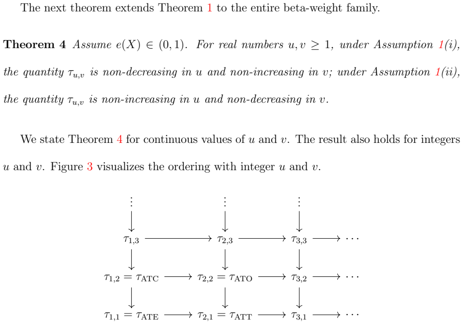
- The bracketing extends beyond ATO to the entire beta-weight family (which includes ATE, ATT, ATC, and ATO), giving a full lattice of ordering relations under the same P-CATE monotonicity.
- In IV studies with a binary instrument and binary treatment, the analogous bracketing holds for overlap-weighted LATE relative to local ATT and local ATC under monotonicity of the complier P-CATE.
- When the propensity score is linear in covariates, population OLS on treatment and covariates recovers τ_ATO, and population TSLS recovers the overlap-weighted LATE, giving regression-based estimators a clean causal interpretation under the bracketing conditions.
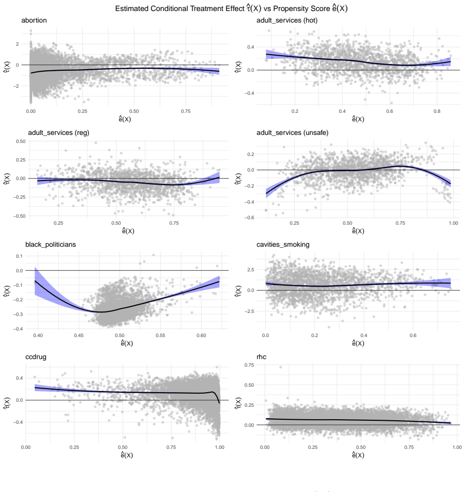
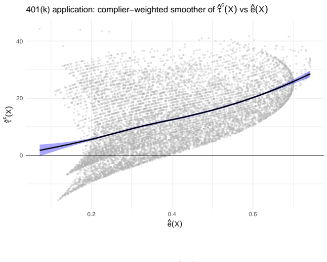
- The CP-plot—estimated CATE versus estimated propensity score—provides a visual check of the monotonicity condition; when the trend is unclear or nonmonotone in the overlap region, the bracketing should not be invoked.
Where Pith is reading between the lines
- The bracketing result could be turned into a sensitivity tool: if an analysis reports only one of ATT, ATO, or ATC, the theorem describes how the estimate would move as the target population shifts, given a monotonic trend.
- The one-crossing theorem suggests a general recipe for comparing any two policy-relevant weights: check whether the normalized weights cross once and whether the P-CATE is monotone in the crossing variable; this could be applied to weights not considered in the paper, such as trimming weights or stabilized weights.
- The connection between linearity of the propensity score and exact equality of OLS/TSLS to overlap-weighted estimands invites a finite-sample version: when estimated propensity scores are approximately linear, regression estimates may be interpreted as approximate overlap-weighted effects without full ignorability.
- A direct testable extension is to estimate the P-CATE function nonparametrically and formally test monotonicity, then use the bracketing result to bound the bias of simpler estimators when monotonicity only holds approximately.
Editorial analysis
A structured set of objections, weighed in public.
Referee Report
Summary. This paper studies ordering relations among weighted average treatment effects under a monotonicity assumption on the P-CATE function g(e)=E{τ(X)|e(X)=e}. Theorem 1 shows that, under Assumption 1(i) (g non-decreasing), τ_ATO lies between τ_ATC and τ_ATT; under Assumption 1(ii) the order reverses. The proof uses covariance/one-crossing representations with zero-mean signed weights. Proposition 1 gives a convex-combination form under linearity (Assumption 2). Section 3 extends the result to local average treatment effects in a binary-IV framework (Theorem 2), and Theorem 3 connects the overlap-weighted LATE to TSLS under a linear IV propensity score. Section 5 generalizes to beta weights (Theorems 4–5) and to a general one-crossing framework (Theorem 6), with matching weights in the supplement. Empirically, the paper introduces a descriptive 'CP-plot' of estimated CATE against estimated propensity score and applies it to eight observational studies and the 401(k) IV example.
Significance. If the results hold, they provide a clean and broadly applicable ordering result for overlap-weighted estimands, filling a gap in the literature. The central derivations are self-contained and the main proof is sound: the pairwise comparisons reduce to E[b(e){g(e)-g(c)}] with zero-mean one-crossing b, so monotonicity of g signs the product. The extension to LATE via the complier-weighted distribution is natural. Assumption 1 is explicitly transparent, and the paper also notes when it fails. The CP-plot is framed as descriptive, not a formal test, which is appropriate. The general beta-weight and one-crossing results extend the scope beyond ATO. The empirical tables are illustrative and consistent with the theory.
minor comments (4)
- [Supplementary B.1 (proof of Theorem 1)] The notation e_l = E{e^l(X)} and e_l = E{(1-e(X))^l} is easily confused with e_l(X). In equations (S2)–(S4) and the definitions of b1 and b2, the expression 'e2(X)' should read 'e(X)^2', with the corresponding denominator 'e2' set in a distinct type (e.g., m_2). As written, b1(x)=e(x)/e1 - e2(x)/e2 is ambiguous.
- [Abstract] The abstract states that the CP-plot is 'implemented in the R package CPplot', but the body of the paper gives no package name, citation, or code-availability statement. Either add a software reference or remove the claim.
- [Section 4 / Table 2] The table and text report that ATO lies between ATT and ATC in every application, but this is a point estimate with substantial sampling uncertainty (e.g., black politicians). The Section 6 caveat is helpful; a one-line note near Table 2 would prevent readers from treating the empirical ordering as a formal confirmation of Assumption 1.
- [Section 5.2, Theorem 6] The theorem is stated for generic weighting functions h and k with E{h}=E{k}. Since earlier sections use normalized weights (e.g., e(X)/E{e(X)}), it would help to state explicitly that Theorem 6 is applied to these normalized weights in the ATT/ATO example that follows.
Circularity Check
No significant circularity: the bracketing theorems are derived algebraically from explicit assumptions, with self-citations only contextual.
full rationale
The derivation chain is self-contained. Theorem 1 is proved in Appendix B.1 by writing τ_ATO − τ_ATT and τ_ATO − τ_ATC as positive constants times E[b_i(X){g(e(X)) − g(c_i)}], where b_i is a zero-mean one-crossing function of the propensity score; the sign of each product is then determined exactly by the explicit monotonicity condition in Assumption 1. Theorem 2 applies the same argument under the complier-weighted distribution E_c, and Theorems 4-6 repeat the same one-crossing comparison for beta weights and general weighting functions. No parameter is fitted to make the conclusion hold, and no 'prediction' is derived from a fitted value: the empirical CP-plots are explicitly described as descriptive diagnostics rather than formal tests, and Tables 2 and 3 report weighted estimates computed by standard formulas while noting that the bracketing follows only under the stated monotonicity. Self-citations, such as Ding (2024), Li et al. (2018, 2019), and Zhao et al. (2026), appear only as background or for regression interpretations, not as load-bearing inputs to the main theorems. The core claim is therefore an ordinary conditional theorem, not a circular reduction.
Axiom & Free-Parameter Ledger
axioms (6)
- domain assumption Potential outcomes framework with binary treatment Z ∈ {0,1} and observed covariates X.
- domain assumption Overlap: e(X) ∈ (0,1).
- domain assumption Assumption 1: g(e) = E{τ(X) | e(X)=e} is either non-decreasing or non-increasing.
- domain assumption Assumption 2: E{τ(X) | e(X)} = a + b e(X) for constants a,b.
- domain assumption Assumption 3: standard binary-IV conditions—conditional IV exogeneity, exclusion restriction, relevance, and monotonicity D(1) ≥ D(0).
- domain assumption Assumption 4: g_c(e) = E{τ_c(X) | U=c, e(X)=e} is either non-decreasing or non-increasing.
Cite this review
Pith. "Pith review of Introducing the CP-plot Based on Covariance Representations of Weighted Average Treatment Effects." pith.science (2026). https://pith.science/paper/LWIPN2H2
@misc{pith2026260611715,
  author       = {Pith},
  title        = {Pith review of: Introducing the CP-plot Based on Covariance Representations of Weighted Average Treatment Effects},
  year         = {2026},
  howpublished = {\url{https://pith.science/paper/LWIPN2H2}},
  note         = {Machine review of arXiv:2606.11715}
}
read the original abstract
Under the canonical setting of observational studies for causal inference, we derive a set of exact representations for pairwise differences among weighted average treatment effects as covariances between the conditional average treatment effect and the propensity score, up to positive scaling factors. These covariance representations immediately imply that (i) the average treatment effect is bracketed by the average treatment effects on the treated and on the controls, with the direction determined by the sign of the covariance between the conditional average treatment effect and the propensity score, and (ii) the average treatment effect under the overlap weight, the weight that is proportional to the conditional variance of the treatment given the covariates, is bracketed by the average treatment effects on the treated and controls when the corresponding covariances have a common sign within both the treated and control groups. We further extend these results to weighted local average treatment effects in the instrumental variable framework. Building on this theory, we recommend the ``CP-plot'' of the estimated conditional average treatment effect against the estimated propensity score, and implement it in the R package CPplot.
Figures
Forward citations
Cited by 1 Pith paper
-
On regression with estimated covariates and conditional effects given the propensity score
New debiased estimators for regression on an estimated propensity score can approach oracle rates, with the corrected plug-in reaching n^{-2/5} under explicit accuracy conditions.
Reference graph
Works this paper leans on
-
[1]
= e1[(1−e 1)(e2 −e 3)−(e 1 −e 2)2] (e1 −e 2)(e2 −e 2
-
[2]
LetA= 1−e(X)andB=e(X)
Becausee 2 −e 2 1 = var{e(X)}, we have λ= E{e(X)}[E{1−e(X)}E[e 2(X){1−e(X)}]−E[e(X){1−e(X)}] 2] E[e(X){1−e(X)}]var{e(X)} . LetA= 1−e(X)andB=e(X). By the definition c∗ = E(AB) E(A) , we have E(A)E(AB2)− {E(AB)}2 =E(A) E(AB2)−2c ∗E(AB) + (c∗)2E(A) =E(A)E{A(B−c ∗)2}. Returning toA= 1−e(X)andB=e(X), this gives E{1−e(X)}E[e 2(X){1−e(X)}]−E[e(X){1−e(X)}] 2 =E{1...
This paper was first reviewed by deepseek-v4-flash on August 2, 2026.
discussion (0)
Sign in with ORCID, Apple, or X to comment. Anyone can read and Pith papers without signing in.