REVIEW 2 major objections 6 minor 1 cited by
Using the wrong orthogonal basis for Volterra identification costs a closed-form excess risk that vanishes exactly when the input is symmetric.
Reviewed by Pith at T0; open to challenge. T0 means a machine referee read the full paper against a public rubric. the ladder, T0–T4 →
T0 review · grok-4.5
2026-07-12 14:13 UTC pith:WM4QBLN6
load-bearing objection Clean closed-form skew penalty for mismatched Wiener diagonals; basis is classical aPC, but the paper owns that and ships a tight Prop. 4 plus Lean and de-confounded experiments. the 2 major comments →
A Closed-Form Skew Penalty for Volterra Cross-Correlation Identification under Non-Gaussian Input
The pith
A machine-rendered reading of the paper's core claim, the machinery that carries it, and where it could break.
Core claim
When a degree-2 signal is expanded in the distribution-matched orthonormal basis, the self-normalized diagonal estimator that instead uses the variance-matched Gaussian (Wiener) features incurs the excess risk (γ₂λ)² + (γ₂ρ − β₂)², where λ = μ₃/σ and γ₂ is the explicit skew-weighted mixing coefficient. The penalty vanishes for every non-degenerate signal if and only if μ₃ = 0.
What carries the argument
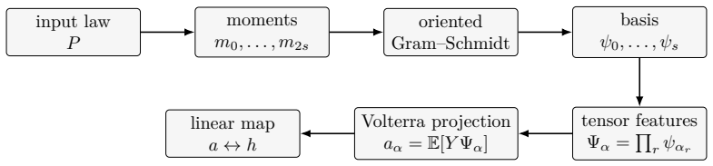
The order-2 misspecification-penalty formula (Proposition 4) together with the oriented Gram–Schmidt VWK basis: the unique positive-leading orthonormal polynomials generated by the input moments, tensorized across independent lags so that diagonal cross-correlation recovers the projection coefficients.
Load-bearing premise
The lagged inputs are treated as independent and identically distributed; if successive lags are correlated, the tensor product basis loses orthonormality and the diagonal estimator is no longer exact.
What would settle it
Generate a degree-2 signal under a centered exponential input, run the self-normalized Gaussian diagonal estimator, and check whether the observed excess risk equals the closed-form value 0.5 predicted by the formula for the paper’s parameters; any systematic deviation falsifies the penalty theorem.
Editorial analysis
A structured set of objections, weighed in public.
Referee Report
Summary. The paper constructs a distribution-matched Volterra–Wiener–Kunchenko (VWK) orthonormal polynomial basis via oriented Gram–Schmidt in L²(P) and applies it as an arbitrary-polynomial-chaos coordinate system for finite-memory Volterra identification under product input laws. The analytic core is Proposition 4: for a degree-2 signal written in the matched basis, the self-normalized variance-matched Gaussian/Wiener diagonal estimator incurs a closed-form excess L²(P) risk (γ₂λ)²+(γ₂ρ−β₂)² governed by the skew coefficient δ=μ₃/σ², vanishing for every nondegenerate signal iff μ₃=0. Supporting material includes a coefficient bijection between monomial and matched coordinates, conditioning diagnostics that separate the population identity Gram from the finite-sample design Gram, a machine-checked Lean 4 proof of the Binomial(N,p)→Krawtchouk row for arbitrary N, and synthetic/real-world experiments that de-confound diagonal projection from full least squares. The authors explicitly disclaim universal prediction superiority and restrict the analysis to moment-based, finite-memory, product-input regimes.
Significance. If Proposition 4 holds as stated—and the derivation from the explicit g₂↔(ψ₁,ψ₂) change of basis plus orthonormality appears tight—the paper supplies a clean, parameter-light account of what the classical Lee–Schetzen/Wiener cross-correlation estimator loses under asymmetric input. That closed form, the machine-checked Krawtchouk instance, the reproducible de-confounding of span versus estimator (full LS identical across bases; large W/V only under skew for diagonal fits), and the honest separation of population versus empirical Gram conditioning are genuine strengths. The contribution is not the matched basis itself (classical aPC/gPC) but the Volterra-estimation reading and the quantified misspecification cost. Within the declared scope this is a useful, carefully scoped addition to non-Gaussian Volterra identification rather than a sweeping methodological overhaul.
major comments (2)
- [Section 7, Proposition 4 / Abstract] Proposition 4 (Section 7, Eq. (1)) is a univariate order-2 result: the excess-risk identity uses only the scalar change-of-basis g₂=(ρψ₂+λψ₁)/(σ²√2) and orthonormality of {ψ₁,ψ₂}. The abstract and introduction present this as the lead contribution for “finite-memory Volterra identification,” yet the multi-lag case (tensor features Ψ_α, d=3 experiments in §9.5–9.6 and Table 8) has no analogous closed-form penalty—only empirical W/oracle and W/emp ratios. Either derive a multi-index extension of (1) under product Pd, or revise the abstract/intro framing so that the analytic claim is clearly univariate order-2 and the finite-memory material is labeled diagnostic/experimental.
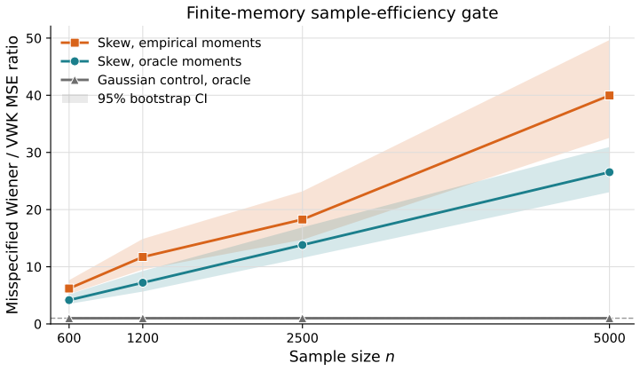
- [Section 9.5, Table 8 / Figure 2] Table 8 and Figure 2 show that empirical-moment VWK can beat oracle VWK even in the Gaussian control (W/emp=1.367 while W/oracle=1). The text attributes this to adaptation to the realized design, but that mechanism is not quantified and blurs the interpretation of the finite-memory “misspecification penalty.” A short analysis (or ablation) of when the empirical basis gains from design adaptation versus when moment estimation error dominates would make the finite-memory claims load-bearing rather than suggestive.
minor comments (6)
- [Table 4 / Remark 2] Table 4 reports sub-nominal β₂ coverage (0.875) under centered-exponential skew. Remark 2 correctly flags finite-sample plug-in SE behavior, but a one-sentence note in the table caption or §9.2 that coverage is diagnostic of the variance estimator—not of Prop. 4—would prevent misreading.
- [Section 9.4, Table 7] Table 7 (ridge diagnostic) shows that CV-tuned η can reverse the fixed-η advantage (centered-exponential s=5 ratio 0.58). The discussion already cautions against overclaiming; consider moving the CV column into the main narrative of §9.4 rather than leaving it as a table-only caveat.
- [Table 1 / Proposition 4] Notation table (Table 1) introduces ρ with “ρ²=μ₄−σ⁴−μ₃²/σ²≥0” then uses ρ as a positive square root in Prop. 4. A single clarifying line that ρ:=√ρ² would remove ambiguity in Eq. (1).
- [Section 2] Related work (§2) cites Carini–Sicuranza and Cheng et al. on distribution-matched orthogonal polynomial filters; a sharper one-paragraph contrast of what those works already achieve for diagonal estimation versus what Prop. 4 newly quantifies would help priority-conscious readers.
- [Section 10, Table 9] The real-world screen (Table 9) is appropriately labeled diagnostic, but the residual-skew columns are training residuals from a monomial span fit, not driver moments. A footnote restating that distinction would avoid conflation with the δ of Prop. 4.
- [Introduction / References] Minor typography: “Thispapertakesthematchedcoordinatesystem” (p. 2, line break artifact) and “EstemPMM” package name in the references should be cleaned in production.
Circularity Check
No significant circularity: Prop. 4 excess-risk formula is a direct L2(P) change-of-basis calculation; population Gram = I is labeled constructional, not sold as evidence.
full rationale
The paper’s analytic core (Proposition 4) derives the closed-form excess L2(P) risk of the self-normalized variance-matched Gaussian diagonal estimator from the explicit order-2 change of basis g2 = (ρψ2 + λψ1)/(σ²√2) and orthonormality of {ψ1, ψ2} under P. The matched projection recovers f exactly only because f is expanded in the orthonormal matched basis—standard Hilbert-space projection, not a hidden fit. The identity Ts Hs T⊤s = I is stated as constructional and is deliberately separated from the finite-sample design Gram reported in Table 6. Synthetic signals are written in the matched basis by design so that W/V isolates basis mismatch; this is disclosed experimental protocol, not a free parameter fitted and then “predicted.” Classical Askey/Hermite reductions follow from uniqueness of oriented orthonormal polynomials (Lemma 1), a standard fact, and the Binomial→Krawtchouk row is machine-checked in Lean 4. Self-citations to Kunchenko/PMM are interpretive and not load-bearing for the penalty identity. Full least squares is correctly declared basis-invariant, so no prediction superiority is claimed by renaming. Within the stated moment-based, product-input scope the derivation chain does not reduce to its inputs by construction.
Axiom & Free-Parameter Ledger
free parameters (1)
- optional ridge level η =
10^{-2} relative or validation-tuned
axioms (5)
- domain assumption Raw moments m0..m2s exist and Hankel Hs is positive definite (monomials linearly independent in L2(P)).
- domain assumption Finite-memory lag vector has product law Pd (independent coordinates).
- standard math Existence and uniqueness of orthonormal polynomials from a positive-definite moment sequence (oriented Gram–Schmidt).
- domain assumption Degree-2 nondegeneracy ρ² > 0 so ψ2 exists (excludes two-point laws).
- ad hoc to paper Finite-sample self-normalized diagonal estimator uses P-norms of Gaussian features, not classical Gaussian normalizing constants.
invented entities (1)
-
Volterra–Wiener–Kunchenko (VWK) basis
independent evidence
read the original abstract
The monomial parameterization of finite-memory Volterra identification is ill-conditioned under non-Gaussian input, and the Wiener--Hermite expansion removes this ill-conditioning only for Gaussian white-noise input. We construct the distribution-matched Volterra--Wiener--Kunchenko (VWK) basis by oriented Gram--Schmidt orthogonalization of monomials in $L^2(P)$ and use it as an arbitrary-polynomial-chaos coordinate system for finite-memory Volterra identification from data, following the generalized polynomial chaos of Xiu and Karniadakis (2002) and the data-driven arbitrary polynomial chaos of Oladyshkin and Nowak (2012). The basis itself is classical; the contribution is the Volterra-estimation reading. First, an order-2 misspecification-penalty theorem shows that a self-normalized diagonal estimator in the variance-matched Gaussian basis incurs an excess $L^2(P)$ risk governed by the skew coefficient $\delta=\mu_3/\sigma^2$, vanishing exactly for symmetric inputs. Second, conditioning experiments separate the constructional fact that the population matched Gram is the identity from the finite-sample design Gram: at $n=2000$, the centered-exponential empirical VWK Gram remains far better conditioned than the power Gram, although it degrades with degree. Third, a machine-checked Lean 4 proof establishes the Binomial$(N,p)$ Krawtchouk row for arbitrary $N$. Full least squares over a fixed span is basis-invariant, so VWK stabilizes diagonal cross-correlation and regularized coordinate fits rather than claiming universal prediction superiority. The analysis is moment-based, finite-memory, and restricted to product input laws.
Figures
Forward citations
Cited by 1 Pith paper
-
Exact Computation of Non-Gaussian Mismatch Penalties in Wiener-Hermite Cross-Correlation Identification
Using a Gaussian Hermite basis under a non-Gaussian input produces an exactly quantifiable mismatch penalty, computable in O(s^3) from moments through order 2s.
Reference graph
Works this paper leans on
-
[1]
Géraud Blatman and Bruno Sudret. Adaptive sparse polynomial chaos expansion based on least angle regression.Journal of Computational Physics, 230(6):2345–2367, 2011. https://doi.org/10.1016/j.jcp.2010.12.021
-
[2]
Brillinger
David R. Brillinger. An introduction to polyspectra.The Annals of Mathematical Statistics, 36(5):1351–1374, 1965
1965
-
[3]
Brillinger.Time Series: Data Analysis and Theory
David R. Brillinger.Time Series: Data Analysis and Theory. Holt, Rinehart and Winston, New York, 1975
1975
-
[4]
R. H. Cameron and W. T. Martin. The orthogonal development of non-linear functionals in series of Fourier–Hermite functionals.Annals of Mathematics, 48(2):385–392, 1947. https://doi.org/10.2307/1969178
doi:10.2307/1969178 1947
-
[5]
Ricardo J. G. B. Campello, Gérard Favier, and Wagner Caradori do Amaral. Optimal expansions of discrete-time Volterra models using Laguerre functions.Automatica, 40(5): 815–822, 2004. https://doi.org/10.1016/j.automatica.2003.11.016
-
[6]
Alberto Carini and Giovanni L. Sicuranza. Selection of a closed-form expression polynomial orthogonal basis for robust nonlinear system identification.Journal of Signal Processing Systems, 2014. https://doi.org/10.1007/s11265-014-0948-2
-
[7]
Alberto Carini, Stefania Cecchi, Laura Romoli, and Giovanni L. Sicuranza. Legendre nonlin- ear filters.Signal Processing, 109:84–94, 2015. https://doi.org/10.1016/j.sigpro.2014.10.037
-
[8]
Generalization of GMM to a continuum of moment conditions.Econometric Theory, 16(6):797–834, 2000
Marine Carrasco and Jean-Pierre Florens. Generalization of GMM to a continuum of moment conditions.Econometric Theory, 16(6):797–834, 2000
2000
-
[9]
C. M. Cheng, Z. K. Peng, W. M. Zhang, and G. Meng. Volterra-series-based nonlinear system modeling and its engineering applications: A state-of-the-art review.Mechanical Systems and Signal Processing, 87:340–364, 2017. https://doi.org/10.1016/j.ymssp.2016.10.029
-
[10]
Chihara.An Introduction to Orthogonal Polynomials
Theodore S. Chihara.An Introduction to Orthogonal Polynomials. Gordon and Breach, New York, 1978
1978
-
[11]
Ernst, Antje Mugler, Hans-Jörg Starkloff, and Elisabeth Ullmann
Oliver G. Ernst, Antje Mugler, Hans-Jörg Starkloff, and Elisabeth Ullmann. On the convergence of generalized polynomial chaos expansions.ESAIM: Mathematical Modelling and Numerical Analysis, 46(2):317–339, 2012. https://doi.org/10.1051/m2an/2011045
-
[12]
On the efficiency of empirical characteristic function procedures.Journal of the Royal Statistical Society: Series B, 43(1):20–27, 1981
Andrey Feuerverger and Philip McDunnough. On the efficiency of empirical characteristic function procedures.Journal of the Royal Statistical Society: Series B, 43(1):20–27, 1981
1981
-
[13]
Advances in Industrial Control
Luigi Fortuna, Salvatore Graziani, Alessandro Rizzo, and Maria Gabriella Xibilia.Soft Sensors for Monitoring and Control of Industrial Processes. Advances in Industrial Control. Springer, London, 2007. https://doi.org/10.1007/978-1-84628-480-9
-
[14]
Walter Gautschi. On generating orthogonal polynomials.SIAM Journal on Scientific and Statistical Computing, 3(3):289–317, 1982. https://doi.org/10.1137/0903018
doi:10.1137/0903018 1982
-
[15]
Roger G. Ghanem and Pol D. Spanos.Stochastic Finite Elements: A Spectral Approach. Springer-Verlag, New York, 1991. https://doi.org/10.1007/978-1-4612-3094-6. 18
-
[16]
Large sample properties of generalized method of moments estimators
Lars Peter Hansen. Large sample properties of generalized method of moments estimators. Econometrica, 50(4):1029–1054, 1982
1982
-
[17]
Peter J. Huber. Robust estimation of a location parameter.The Annals of Mathematical Statistics, 35(1):73–101, 1964
1964
-
[18]
Heysem Kaya, Pınar Tüfekci, and Erdinç Uzun. Predicting CO and NOx emissions from gas turbines: novel data and a benchmark PEMS.Turkish Journal of Electrical Engineering and Computer Sciences, 27(6):4783–4796, 2019. https://doi.org/10.3906/elk-1807-87
-
[19]
Vassilis Kekatos and Georgios B. Giannakis. Sparse Volterra and polynomial regression models: Recoverability and estimation.IEEE Transactions on Signal Processing, 59(12): 5907–5920, 2011. https://doi.org/10.1109/TSP.2011.2165952
-
[20]
Lesky, and René F
Roelof Koekoek, Peter A. Lesky, and René F. Swarttouw.Hypergeometric Orthogonal Polynomials and Their q-Analogues. Springer Monographs in Mathematics. Springer, Berlin, 2010
2010
-
[21]
Michael J. Korenberg. Identifying nonlinear difference equation and functional expansion representations: The fast orthogonal algorithm.Annals of Biomedical Engineering, 16(1): 123–142, 1988. https://doi.org/10.1007/BF02367385
-
[22]
Y. P. Kunchenko.Polynomial Parameter Estimations of Close to Gaussian Random Variables. Shaker Verlag, Aachen, 2002
2002
-
[23]
Y. P. Kunchenko.Stochastic Polynomials. Naukova Dumka, Kyiv, 2006
2006
-
[24]
Y. W. Lee and M. Schetzen. Measurement of the Wiener kernels of a non-linear system by cross-correlation.International Journal of Control, 2(3):237–254, 1965
1965
-
[25]
Marmarelis.Nonlinear Dynamic Modeling of Physiological Systems
Vasilis Z. Marmarelis.Nonlinear Dynamic Modeling of Physiological Systems. Wiley-IEEE Press, Hoboken, NJ, 2004
2004
-
[26]
John Mathews and Giovanni L
V. John Mathews and Giovanni L. Sicuranza.Polynomial Signal Processing. Wiley, New York, 2000
2000
-
[27]
Nikias and Athina P
Chrysostomos L. Nikias and Athina P. Petropulu.Higher-Order Spectra Analysis: A Nonlinear Signal Processing Framework. Prentice Hall, Englewood Cliffs, NJ, 1993
1993
-
[28]
Sergey Oladyshkin and Wolfgang Nowak. Data-driven uncertainty quantification using the arbitrary polynomial chaos expansion.Reliability Engineering & System Safety, 106: 179–190, 2012. https://doi.org/10.1016/j.ress.2012.05.002
-
[29]
Wiley, New York, 1980
Martin Schetzen.The Volterra and Wiener Theories of Nonlinear Systems. Wiley, New York, 1980
1980
-
[30]
Wim Schoutens.Stochastic Processes and Orthogonal Polynomials, volume 146 ofLecture Notes in Statistics. Springer, New York, 2000. https://doi.org/10.1007/978-1-4612-1170-9
-
[31]
Christian Soize and Roger Ghanem. Physical systems with random uncertainties: Chaos representations with arbitrary probability measure.SIAM Journal on Scientific Computing, 26(2):395–410, 2004. https://doi.org/10.1137/S1064827503424505
-
[32]
Ameri- can Mathematical Society, Providence, RI, 1939
Gábor Szegő.Orthogonal Polynomials, volume 23 ofAMS Colloquium Publications. Ameri- can Mathematical Society, Providence, RI, 1939. 19
1939
-
[33]
Emiliano Torre, Stefano Marelli, Paul Embrechts, and Bruno Sudret. Data-driven polynomial chaos expansion for machine learning regression.Journal of Computational Physics, 388: 601–623, 2019. https://doi.org/10.1016/j.jcp.2019.03.039
-
[34]
Blackie, London, 1930
Vito Volterra.Theory of Functionals and of Integral and Integro-Differential Equations. Blackie, London, 1930
1930
-
[35]
Xiaoliang Wan and George Em Karniadakis. Beyond Wiener–Askey expansions: Handling arbitrary PDFs.Journal of Scientific Computing, 27(1–3):455–464, 2006. https://doi.org/10.1007/s10915-005-9038-8
-
[36]
MIT Press, Cambridge, MA, 1958
Norbert Wiener.Nonlinear Problems in Random Theory. MIT Press, Cambridge, MA, 1958
1958
-
[37]
Jeroen A. S. Witteveen and Hester Bijl. Modeling arbitrary uncertainties using gram-schmidt polynomial chaos. In44th AIAA Aerospace Sciences Meeting and Exhibit. American Institute of Aeronautics and Astronautics, 2006. https://doi.org/10.2514/6.2006-896
-
[38]
The Wiener–Askey polynomial chaos for stochastic differential equations.SIAM Journal on Scientific Computing, 24(2):619–644,
Dongbin Xiu and George Em Karniadakis. The Wiener–Askey polynomial chaos for stochastic differential equations.SIAM Journal on Scientific Computing, 24(2):619–644,
-
[39]
https://doi.org/10.1137/S1064827501387826
-
[40]
Empirical characteristic function estimation and its applications.Econometric Reviews, 23(2):93–123, 2004
Jun Yu. Empirical characteristic function estimation and its applications.Econometric Reviews, 23(2):93–123, 2004
2004
-
[41]
S. W. Zabolotnii, Z. L. Warsza, and O. Tkachenko. Polynomial estimation of linear regression parameters for the asymmetric pdf of errors. InAdvances in Intelligent Systems and Computing, volume 743, pages 709–722. Springer, 2018
2018
-
[42]
EstemPMM: Polynomial maximization method estimation
Serhii Zabolotnii. EstemPMM: Polynomial maximization method estimation. https: //cran.r-project.org/package=EstemPMM, 2026. R package version 0.4.0
2026
-
[43]
Serhii V. Zabolotnii. From Volterra series to Kunchenko stochastic polynomials: Half a century of non-Gaussian estimation methodology. arXiv preprint arXiv:2605.22354, 2026. 20
Pith/arXiv arXiv 2026
discussion (0)
Sign in with ORCID, Apple, or X to comment. Anyone can read and Pith papers without signing in.