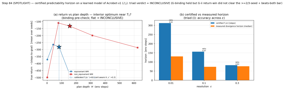
Certified World Models: Predictability Across Configuration, Horizon, and Resolution
Pith reviewed 2026-07-03 23:57 UTC · model grok-4.3
The pith
Equivariant world models certify rollout error bounds from symmetry generators and Lyapunov spectra across configurations, horizons, and resolutions.
A machine-rendered reading of the paper's core claim, the machinery that carries it, and where it could break.
Core claim
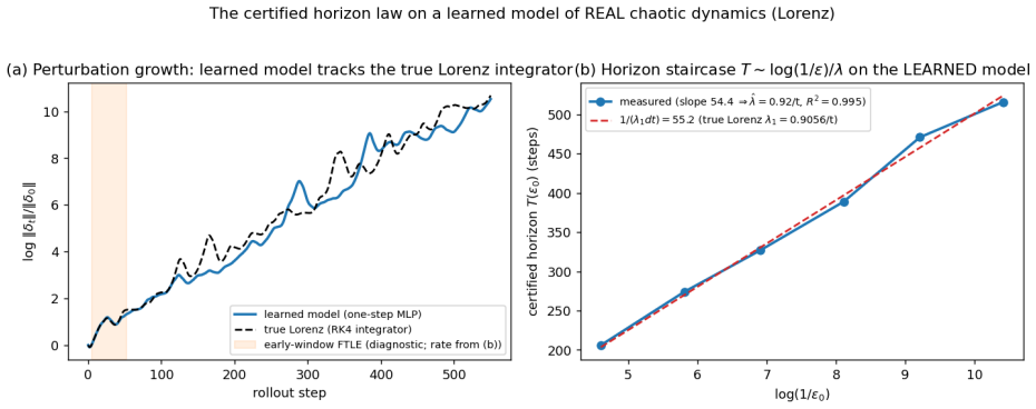
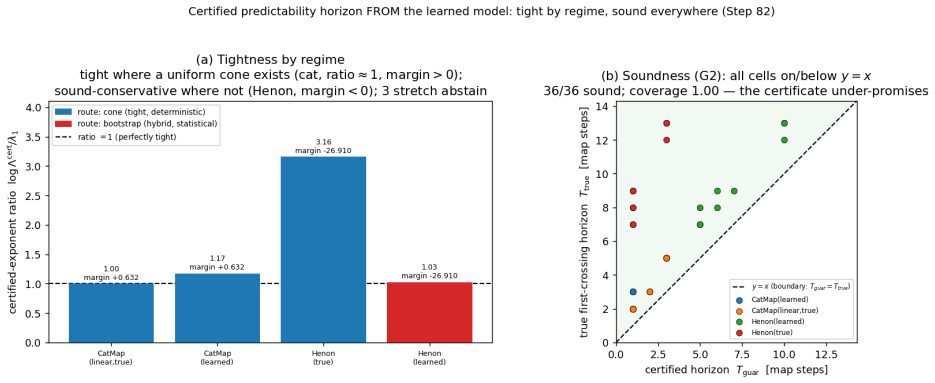
Under exact equivariance, rollout error is invariant over the monoid generated by k primitive symmetries and is certified from the k generators (Theorem A). Approximate orbit-transfer defects propagate by the finite-time Lyapunov spectrum (Theorem B): expanding channels give logarithmic horizons, neutral channels accumulate defect linearly, and contracting channels accumulate a bounded floor. Exact conserved charges are certified to all horizons only at zero defect; with one-step defect eta, charge error grows at most as T eta. A cone certificate from the Jacobian supplies a configuration-dependent horizon that is tight on uniformly hyperbolic dynamics.
What carries the argument
The predictability certificate that combines exact invariance under symmetry monoids with propagation of one-step orbit defects via the finite-time Lyapunov spectrum of the model Jacobian.
If this is right
- Rollout trustworthiness becomes computable from the generators and Jacobian without simulating the full trajectory.
- Horizons scale logarithmically with error tolerance in expanding directions and linearly in neutral directions.
- Conserved quantity errors remain bounded by T times the one-step defect.
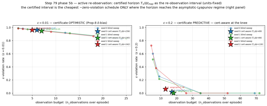
- A budgeted re-observation policy can use the cone certificate to decide when to trust the model or request new data.
- Non-equivariant models can still obtain a training-free candidate horizon from the tangent spectrum together with a held-out divergence check.
Where Pith is reading between the lines
- The certificate could be combined with model-based control to abstain from actions whose predicted trajectories exceed the certified horizon.
- The same Jacobian-based propagation idea might extend to models with other known structure such as conservation laws or Lie-group symmetries.
- Training objectives could be augmented to minimize not only prediction loss but also the size of the one-step orbit defects that limit the certified horizon.
- On physical systems whose symmetries are known a priori, the recovered Lyapunov spectrum could be compared against analytic expectations to test whether the learned model has captured the correct local geometry.
Load-bearing premise
The world model is either exactly equivariant or its one-step orbit-transfer defects can be measured and then propagated through the Jacobian without additional unmodeled error sources.
What would settle it
Run the model on two inputs related by one primitive symmetry and observe whether the rollout errors differ by more than the certified bound when the model is claimed to be exactly equivariant.
Figures


read the original abstract
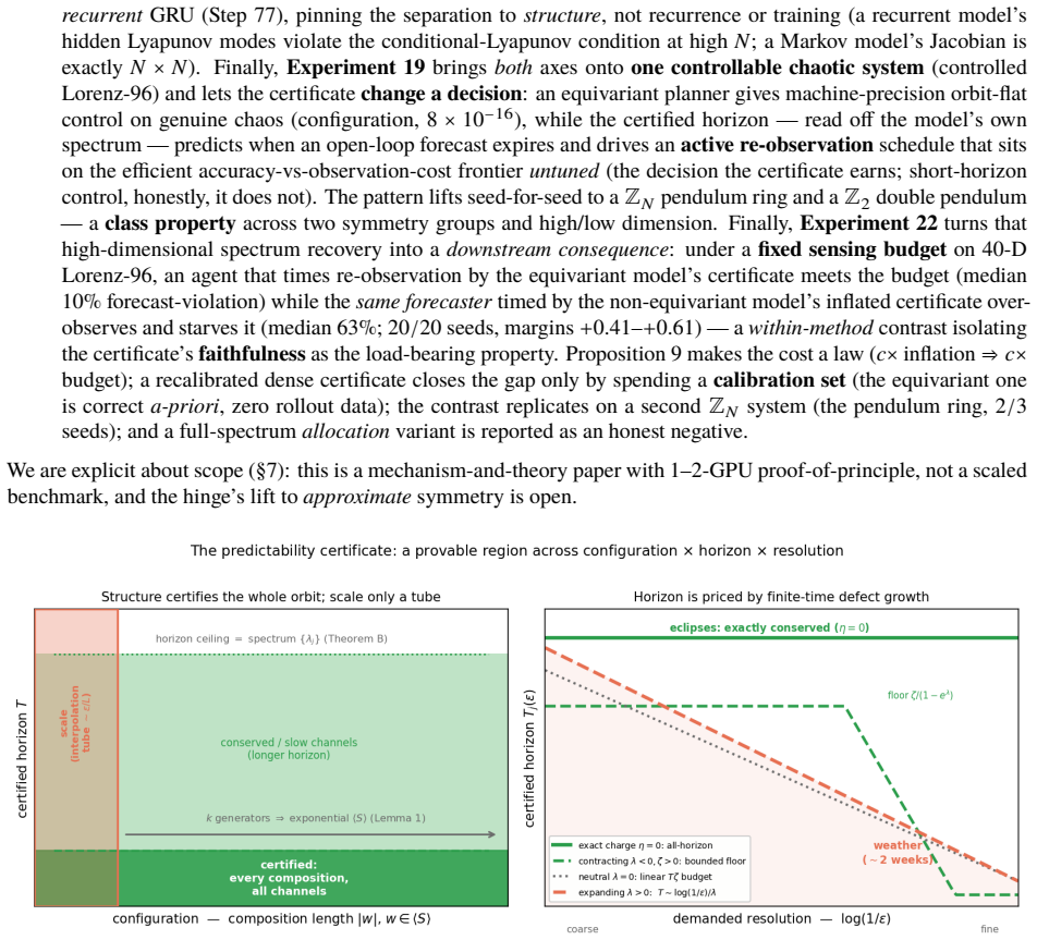
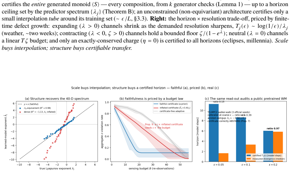
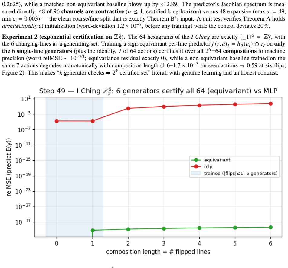
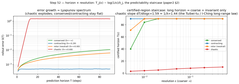
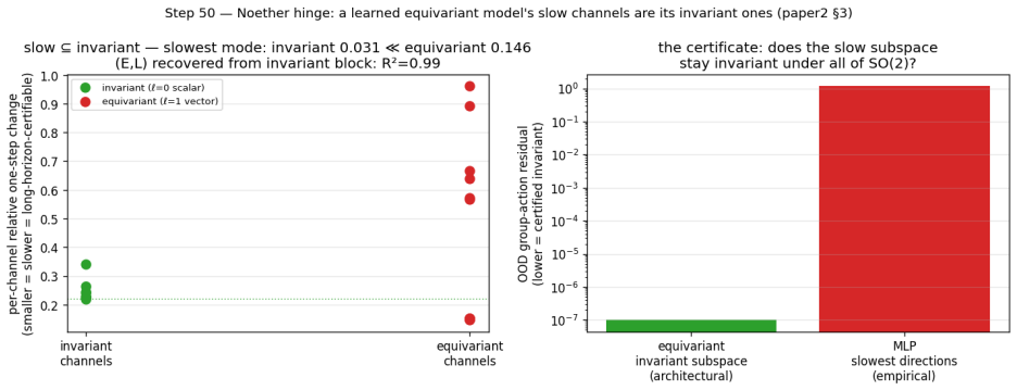
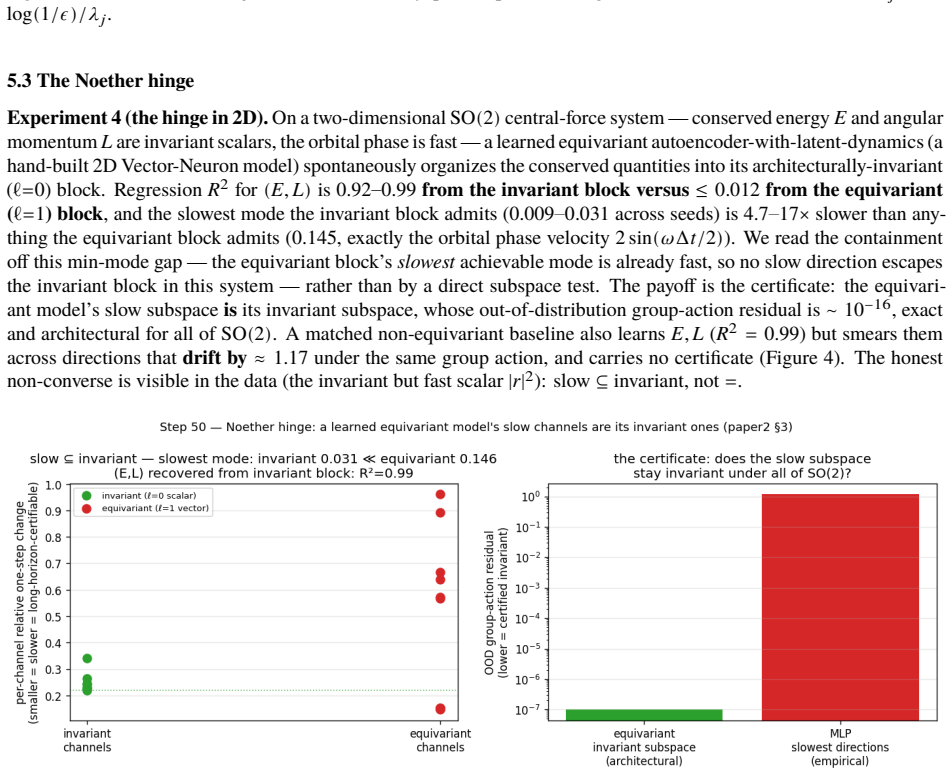
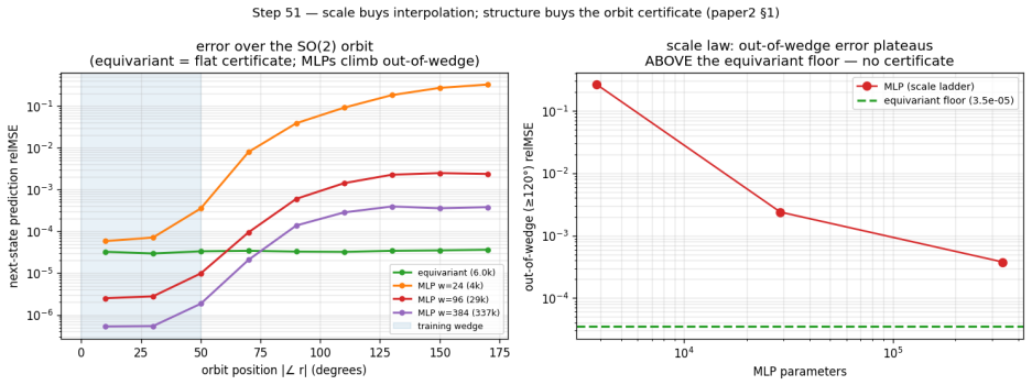
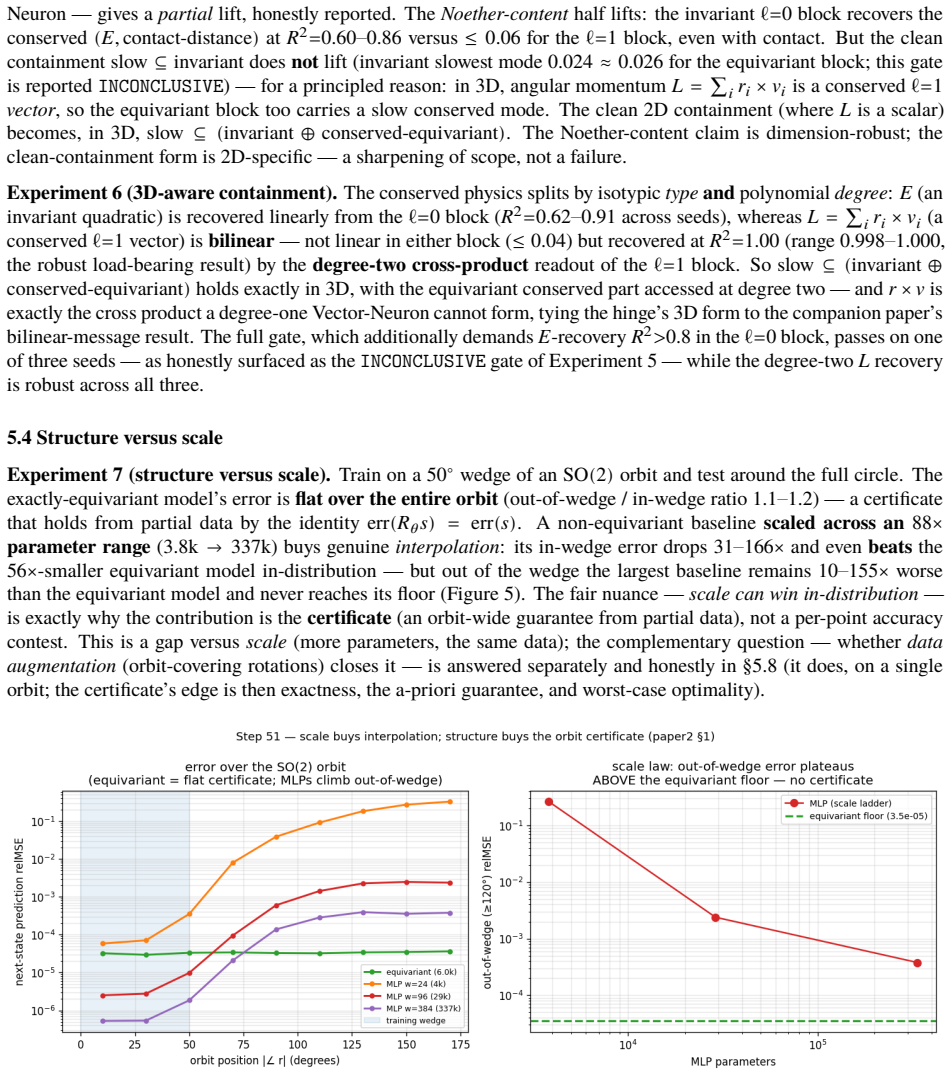
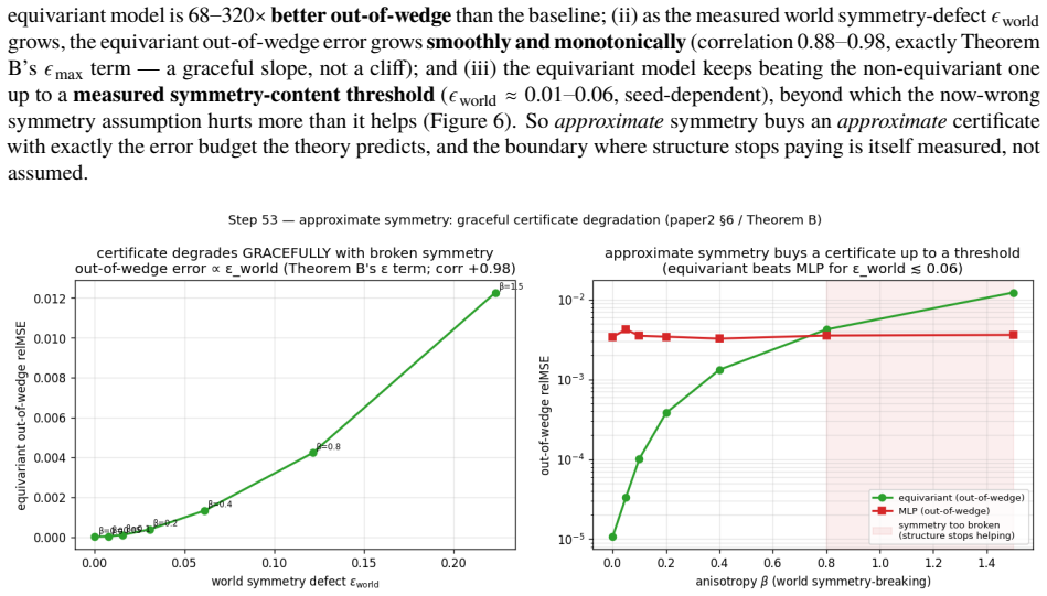
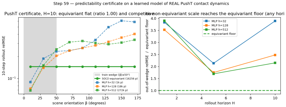
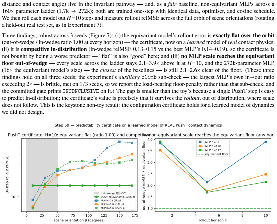
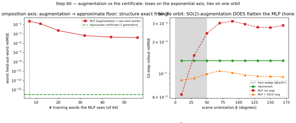
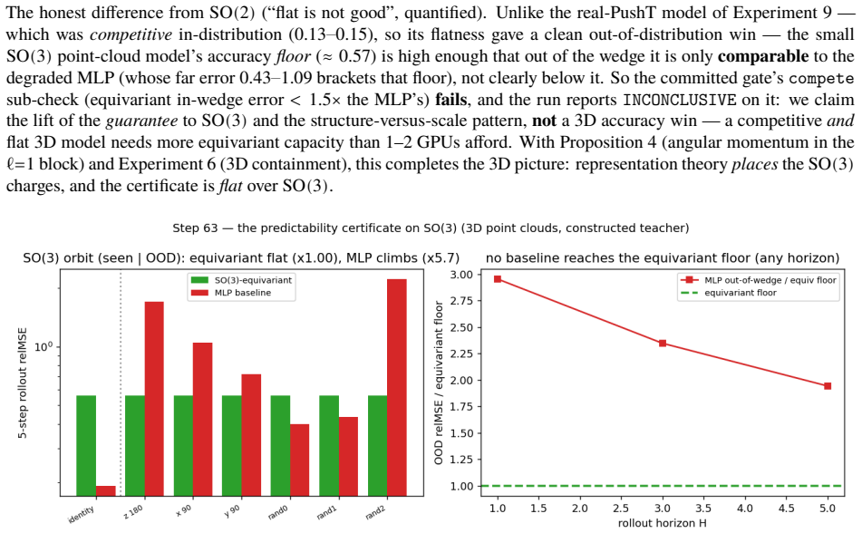
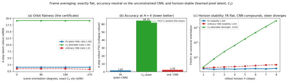
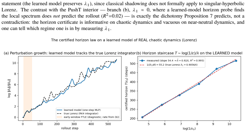
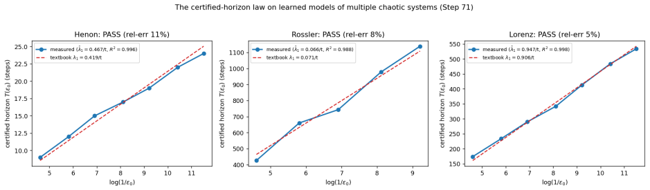
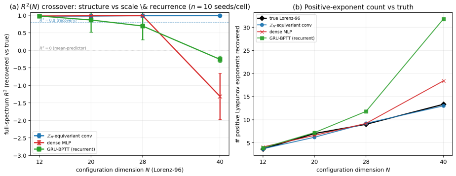
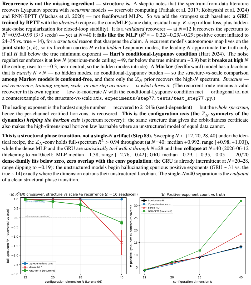
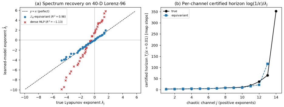
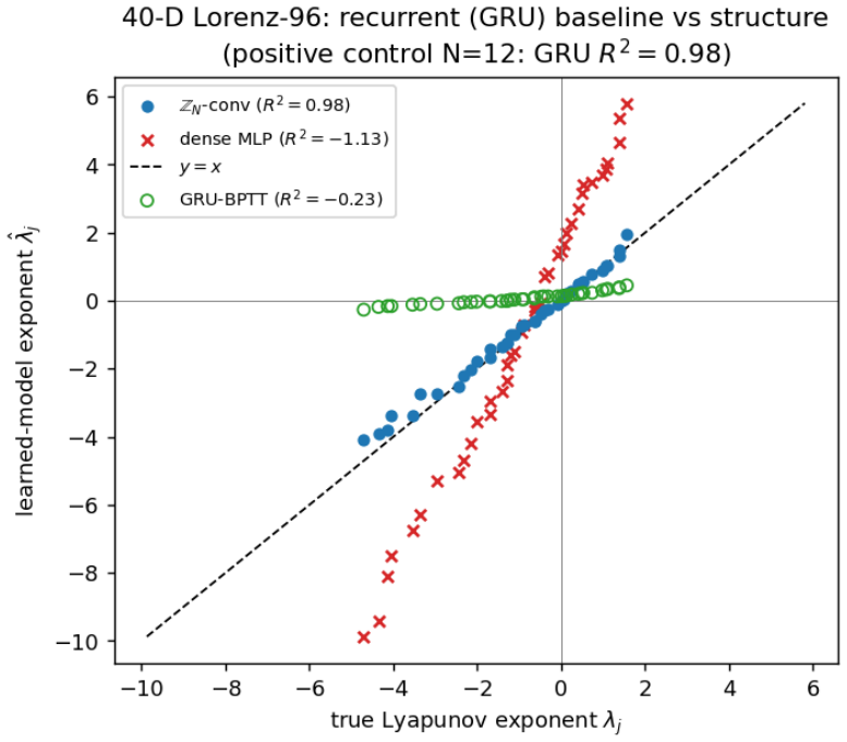
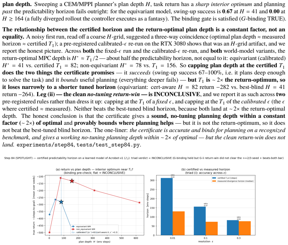
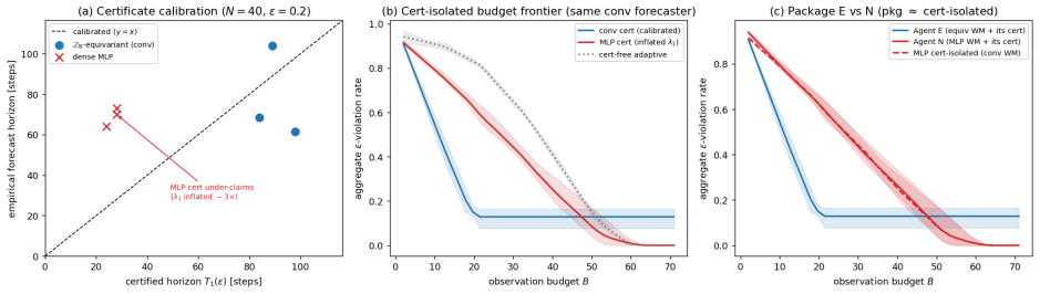
Scale buys interpolation; structure buys certifiable transfer. A world model's average error does not say whether a particular rollout can be trusted, or for how long. For equivariant latent world models we give a predictability certificate: a computable region spanning configuration, horizon, and resolution. Under exact equivariance, rollout error is invariant over the monoid generated by k primitive symmetries and is certified from the k generators (Theorem A); universal orbit-flatness over equivariant targets characterizes equivariance at the function level (Lemma 2), so an unconstrained architecture cannot certify the property by construction. Approximate orbit-transfer defects propagate by the finite-time Lyapunov spectrum (Theorem B): expanding channels give a logarithmic horizon $T_j(\epsilon)\sim\log(1/\epsilon)/\lambda_j$, neutral channels accumulate recurrent defect linearly, and contracting channels accumulate a bounded nonzero floor. Exact conserved charge values are certified to all horizons only at zero defect; with one-step defect $\eta$, charge-value error grows at most as $T\eta$. Empirically, on a 40-dimensional learned model a $\mathbb{Z}_N$-equivariant network recovers the full Lyapunov spectrum ($R^2=0.98$-$0.99$) where dense and recurrent baselines fail. A cone/adapted-metric certificate reads an a-priori horizon off the model's own Jacobian, tight on uniformly hyperbolic dynamics and self-abstaining elsewhere; the resulting horizon improves a budgeted re-observation decision. For public non-equivariant world models the tangent spectrum gives a training-free candidate horizon, paired with a held-out divergence cross-check that abstains or corrects when the learned loop over-promises.
Editorial analysis
A structured set of objections, weighed in public.
Referee Report
Summary. The manuscript claims a predictability certificate for equivariant latent world models spanning configuration, horizon, and resolution. Under exact equivariance, rollout error is invariant over the monoid generated by k primitive symmetries and certified from the k generators (Theorem A); universal orbit-flatness characterizes equivariance (Lemma 2). Approximate orbit-transfer defects propagate via the finite-time Lyapunov spectrum of the Jacobian (Theorem B), yielding logarithmic horizons T_j(ε) ~ log(1/ε)/λ_j for expanding channels, linear accumulation for neutral channels, and bounded floors for contracting channels. Exact conserved charges are certified only at zero defect. Empirically, a Z_N-equivariant network on a 40-dimensional model recovers the full Lyapunov spectrum (R^2=0.98-0.99) while dense and recurrent baselines fail; a cone/adapted-metric certificate reads an a-priori horizon from the model's Jacobian, and a tangent-spectrum approach is offered for non-equivariant models with a divergence cross-check.
Significance. If the theorems and empirical claims hold, the work supplies a structured, Jacobian-derived certificate that goes beyond average error to bound trustworthiness of individual rollouts, which would be a meaningful advance for reliable world models in planning and control. The explicit linkage of equivariance to invariance (Theorem A) and the demonstration that an equivariant architecture recovers the spectrum where baselines do not are concrete strengths; the cone certificate's self-abstaining property on non-hyperbolic dynamics is also a practical feature.
major comments (3)
- [Theorem B] Theorem B: the propagation claim states that one-step orbit-transfer defects are the sole error source whose accumulation is fully captured by the finite-time Lyapunov spectrum, yet the manuscript provides no explicit bounds on Jacobian estimation error or higher-order nonlinear accumulation in the 40-dimensional learned setting; this assumption is load-bearing for both the logarithmic/neutral/contracting horizon formulas and the charge-error bound Tη.
- [Empirical results] Empirical section: the R^2=0.98-0.99 spectrum recovery is reported for the Z_N-equivariant network, but the evaluation does not include a direct test of whether the derived T_j(ε) horizons actually bound observed rollout error under measured one-step defects, leaving the practical tightness of the cone/adapted-metric certificate unverified.
- [Theorem A] Theorem A and Lemma 2: the reduction of the certificate to the k generators under exact equivariance relies on the monoid-invariance property and the orbit-flatness characterization; the manuscript should supply the explicit construction showing how the certificate is computed from the generators alone, as this is central to the claim that unconstrained architectures cannot certify by construction.
minor comments (2)
- The abstract and text use 'adapted-metric certificate' and 'cone' without an inline definition or small illustrative example; adding one would improve readability.
- Notation for the finite-time Lyapunov exponents λ_j and the defect η should be consistently defined with respect to the model's Jacobian before the horizon formulas are stated.
Simulated Author's Rebuttal
We thank the referee for the thorough and constructive report. The three major comments identify substantive gaps in the presentation of the theorems and in the empirical validation. We address each below and indicate where revisions will be made.
read point-by-point responses
-
Referee: [Theorem B] Theorem B: the propagation claim states that one-step orbit-transfer defects are the sole error source whose accumulation is fully captured by the finite-time Lyapunov spectrum, yet the manuscript provides no explicit bounds on Jacobian estimation error or higher-order nonlinear accumulation in the 40-dimensional learned setting; this assumption is load-bearing for both the logarithmic/neutral/contracting horizon formulas and the charge-error bound Tη.
Authors: We agree that Theorem B relies on the linear propagation of one-step defects via the finite-time Lyapunov spectrum and does not supply explicit a-priori bounds on Jacobian estimation error or on the remainder terms arising from nonlinear accumulation. The horizon formulas and the Tη charge-error bound are therefore derived under the stated linear approximation. In the revision we will add a dedicated limitations paragraph that (i) states the small-defect and local-hyperbolicity conditions under which the linearization is justified, (ii) notes that Jacobian estimation error is not bounded in the current proofs, and (iii) clarifies that the cone certificate is self-abstaining precisely when these conditions fail. We view this as a clarification rather than a change to the theorems themselves. revision: partial
-
Referee: [Empirical results] Empirical section: the R^2=0.98-0.99 spectrum recovery is reported for the Z_N-equivariant network, but the evaluation does not include a direct test of whether the derived T_j(ε) horizons actually bound observed rollout error under measured one-step defects, leaving the practical tightness of the cone/adapted-metric certificate unverified.
Authors: The referee correctly observes that the reported experiments validate spectrum recovery but do not close the loop by checking whether the predicted T_j(ε) horizons, computed from measured one-step defects, actually upper-bound the observed rollout error. We will add this verification experiment to the empirical section: for the 40-dimensional model we will (a) record per-channel one-step orbit-transfer defects on a held-out trajectory set, (b) compute the corresponding T_j(ε) horizons from the learned Jacobian, and (c) compare the predicted horizons against the empirically observed error growth. The cone/adapted-metric certificate will be evaluated on the same trajectories to quantify its tightness and abstention behavior. revision: yes
-
Referee: [Theorem A] Theorem A and Lemma 2: the reduction of the certificate to the k generators under exact equivariance relies on the monoid-invariance property and the orbit-flatness characterization; the manuscript should supply the explicit construction showing how the certificate is computed from the generators alone, as this is central to the claim that unconstrained architectures cannot certify by construction.
Authors: We accept that the current proof sketch of Theorem A invokes monoid invariance and orbit-flatness but does not spell out the inductive construction that reduces the certificate to the k primitive generators. In the revised manuscript we will expand the proof of Theorem A with an explicit inductive step: starting from the action of each generator, we show how the invariance of the error functional propagates over arbitrary words in the monoid, thereby demonstrating that the certificate depends only on the k generators and the associated Jacobian spectrum. This construction will also be used to contrast with unconstrained architectures, which lack the generator-level invariance by design. revision: yes
Circularity Check
No significant circularity; theorems derive from standard equivariance and Lyapunov properties with independent empirical checks.
full rationale
The abstract presents Theorem A as invariance certified from symmetry generators under exact equivariance, and Theorem B as defect propagation via the finite-time Lyapunov spectrum of the Jacobian. These are standard dynamical-systems facts applied to the equivariant case, not reductions to fitted inputs or self-citations. The empirical claim (R^2=0.98-0.99 spectrum recovery on a Z_N-equivariant network, with baselines failing) is a comparative test rather than a prediction forced by the architecture. No self-citation load-bearing steps, ansatz smuggling, or renaming of known results appear in the provided text. The derivation chain remains self-contained against external benchmarks.
Axiom & Free-Parameter Ledger
Forward citations
Cited by 1 Pith paper
-
Certified World Models as Sensing Clocks: Drift-Aware Deadlines for Active Perception
Derives a drift-aware sensing clock from certified world models that controls certificate violations on held-out data and outperforms expected-belief scheduling in a synthetic benchmark at matched sensing budget.
Reference graph
Works this paper leans on
-
[1]
— penalizes the latent-transition Jacobian to damp rollout error propagation; the heuristic version of Theorem B’s provable per-channel horizon. arXiv:2501.00195. Classical dynamical-systems results behind the horizon axis (Theorem B, Proposition 7): • Oseledets multiplicative ergodic theorem (Oseledets, 1968) — under an ergodic invariant measure with log...
-
[2]
SO(2)𝑧 approximate (fixed base; Thm A representation regime) 54 Exp
yet has no certificate (Lemma 2). SO(2)𝑧 approximate (fixed base; Thm A representation regime) 54 Exp. Result Code Test Seeds Headline number 17 Certificate at the planning level on FetchPush experiments/step73_ fetchpush_ planning.py tests/test_ step73_ planner_ equivariance.py 3 equivariant WM + equivariant goal-readout head + 𝐺-equivariant CEM: the who...
discussion (0)
Sign in with ORCID, Apple, or X to comment. Anyone can read and Pith papers without signing in.