REVIEW 3 major objections 7 minor 1 cited by
Learning only the boundary correction of Stokes flow keeps the solver exact and makes geometric transfer a question of invariance and coverage.
Reviewed by Pith at T0; open to challenge. T0 means a machine referee read the full paper against a public rubric. the ladder, T0–T4 →
2026-07-12 12:23 UTC pith:Q4UJDDCW
load-bearing objection Clean Stokes testbed that isolates what learning actually buys: amortization of the boundary correction, with invariance and coverage as the real levers for geometric transfer. the 3 major comments →
Solver Exactness, Learned Flexibility: Equivariant Boundary-Correction Operators for Stokes Flow
The pith
A machine-rendered reading of the paper's core claim, the machinery that carries it, and where it could break.
Core claim
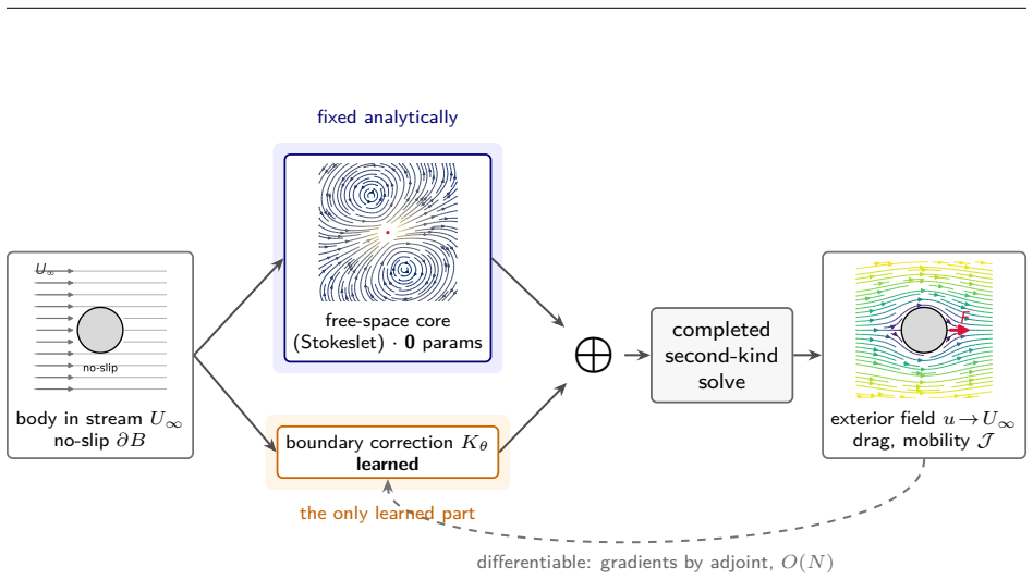
On an exactly solvable Stokes testbed, fixing the free-space Stokeslet core and learning only the boundary correction yields a working end-to-end solver at about 2×10^{-3} interior accuracy that is 5–16× more data-efficient than a black-box DeepONet; geometric generalization is governed by descriptor invariance and training coverage, not by conditioning or capacity. Learning contributes amortization alone—accuracy, differentiability, and O(N) scaling already belong to the solver.
What carries the argument
The rigid-core / learned-boundary split: the free-space Leray projector is the exact Stokeslet (zero parameters, SO(3)-equivariant by construction); only the geometry-dependent boundary correction is learned as a completed second-kind operator, optionally reparameterized as a local equivariant kernel.
Load-bearing premise
The free-space fundamental solution can be absorbed into a rigid exact core so that the only learnable object is a boundary remainder—an assumption that holds for linear Stokes but fails for high-Reynolds nonlinear flow where no such free-space kernel exists.
What would settle it
Train the split and a black-box operator on the same continuous shape distribution and measure held-out interior field error: if the split is not several times more accurate at equal budget, or if a non-invariant descriptor still transfers under free rotation, the central claims fail.
Editorial analysis
A structured set of objections, weighed in public.
Referee Report
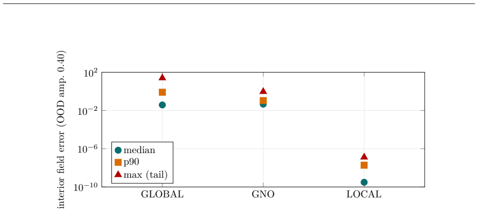
Summary. The paper studies Stokes flow by splitting the solution operator into an exact free-space Stokeslet core (zero learnable parameters, SO(3)-equivariant by construction, O(N) via FMM) and a learned boundary correction with no closed form. On a controlled 2D interior testbed with dense BEM ground truth, the authors show that conditioning is not the learning bottleneck (first- vs second-kind, Table 1), that cross-shape generalization is governed by descriptor invariance and training coverage rather than capacity (Fig. 2, Tables 2–3), that Wielandt completion is necessary for a stable learned solve (Proposition 1), and that an end-to-end pipeline reaches ~2×10^{-3} interior accuracy. Against baselines the split is 5–16× more data-efficient than a black-box DeepONet and ~2.5× better in-distribution than a geometry-aware GNO-style operator, with OOD fragility of the global map removed by a local equivariant kernel. Section 10 opens the 3D exterior problem with a completed QBX double-layer foundation and early learned drag/mobility operators.
Significance. If the results hold, the paper cleanly answers what a learned Stokes operator retains of the classical solver and what controls geometric transfer—questions usually left opaque in black-box operator learning. Strengths include exact dense BIE and analytic (Oberbeck) references rather than finer-grid surrogates, machine-precision equivariance residuals, controlled ablations (conditioning, rotation, discrete vs continuous coverage, global vs local parameterization), Proposition 1 with numerical verification, an honest GNO baseline that narrows the claim, and an explicit scope limit on free-space kernels. The amortization framing (learning buys a one-time train cost, not accuracy, differentiability, or O(N)) is unusually precise. The work is of clear interest to microhydrodynamics and to the operator-learning community as a methodological testbed.
major comments (3)
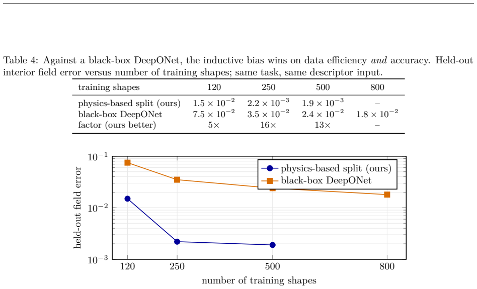
- §9, Table 4 and surrounding text: the 5–16× data-efficiency claim against DeepONet is load-bearing for the abstract and conclusion. The manuscript states the DeepONet is “reasonably tuned but not exhaustively optimized” and that the same canonicalized descriptor is used, but does not report branch/trunk widths, depth, training schedule, or validation that capacity was matched. Without those details the factor is hard to reproduce and the plateau comparison is weaker than the GNO head-to-head that follows. Please add architecture and hyperparameter tables (or an appendix) so the black-box baseline can be audited at the same standard as the GNO.
- §6 (local equivariant kernel) and §9 / Fig. 5: when the radial profile is fit from data alone it recovers the universal coefficient 1/π to ~10^{-11} and extrapolates to machine precision. That is a strong positive result for the inductive bias, but it also means that on the smooth second-kind operator the “learned” map is essentially rediscovering the analytic kernel. The residual frontier is correctly identified as near-field/QBX singular structure, yet the end-to-end OOD claim in Fig. 5 and the abstract (“learned map… reduced… with a local equivariant kernel”) should state explicitly whether the local kernel used in the full pipeline still contains a nontrivial learned remainder or has collapsed to the closed-form double layer. Clarify what is still being learned once locality and equivariance are imposed.
- §10: the 3D exterior foundations (completed QBX double layer, Oberbeck drag match, machine-precision SO(3) equivariance, Lorentz reciprocity) are solid and well scoped as “opening” the problem. The subsequent learned resistance tensor on the ℓ=2 family (five training shapes, ~1.5×10^{-3} held-out) and the exterior-field model are early and on a narrow shape class. Phrases such as “turn the exterior foundations into a working learned program” and the abstract’s SO(3) guarantees risk overstating the learned 3D evidence relative to the carefully quantified 2D interior results. Please either add quantitative tables for 3D drag/mobility comparable to Tables 2–4, or temper the language so that §10 remains clearly foundational plus proof-of-concept.
minor comments (7)
- Abstract and §1: “5 to 16× more data-efficient” and “~2.5× lower in-distribution error” are clear; consider also stating the absolute floors (~2×10^{-3} vs DeepONet plateau ~2×10^{-2}) so readers do not need Table 4 to interpret the factors.
- §4, Table 1: report the network architecture / feature dimension used for “sufficient” vs “reduced” capacity so the capacity ablation is reproducible.
- §5: the horseshoe / near-slit conditioning discussion is valuable; a single figure of the C-shaped geometry and cond(N) would help readers who skip the text.
- §7, Proposition 1: the proof sketch is classical; a one-line pointer to the exact lemma in af Klinteberg et al. (2020) or Pozrikidis (1992) for the left-nullspace claim would tighten the citation.
- §8–9: wall-clock amortization (~50 µs vs ~0.45 s) is useful; state N and hardware so the four-order claim is interpretable.
- References: several arXiv-only entries (PACE-FNO 2026, Meshfree exterior calculus 2026, etc.) are concurrent; ensure final versions or stable arXiv IDs are used at camera-ready.
- Typos / style: “many-particlesuspensions”, “ortheswimming”, “themaccurately”, “splitthe”, “andSO(3)” (missing spaces) appear in the abstract/intro; a global pass for spacing and hyphenation would help.
Circularity Check
No significant circularity: claims rest on independent exact BIE ground truth, classical Stokes structure, and external baselines, not on self-definitional or fitted tautologies.
full rationale
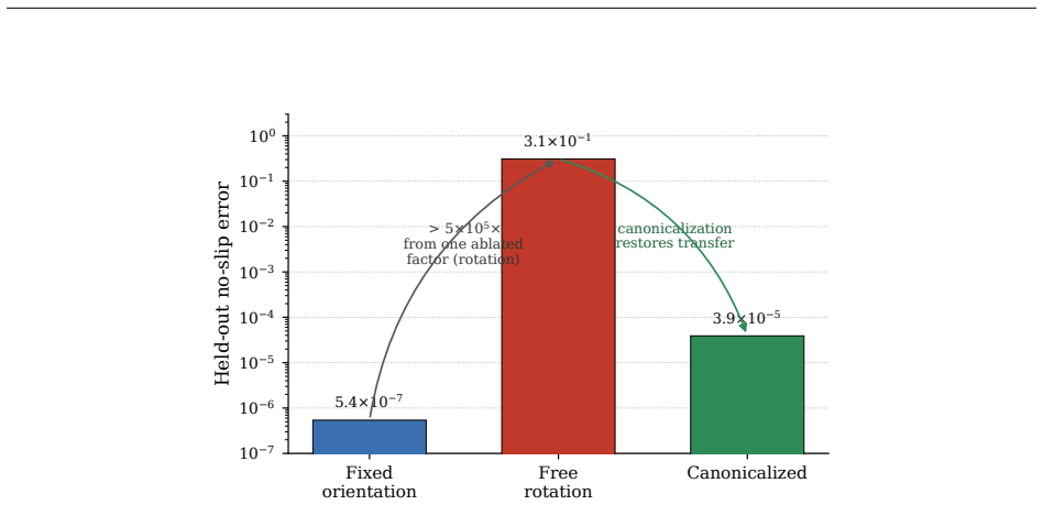
The paper's derivation chain is self-contained against external references. The free-space Stokeslet core (Eq. 1, §3) is the known analytic Oseen tensor, fixed with zero parameters and verified to machine-precision equivariance (~10^{-16}); attempts to fit it recover the closed form rather than inventing it. Boundary-correction learning is trained and measured against an independent dense second-kind BIE solve (the BEM ground truth) or closed-form Oberbeck drag, not against a surrogate of itself. Conditioning ablation (Table 1), rotation/canonicalization ablation (Fig. 2), coverage scaling (Table 2), end-to-end pipeline (~2e-3, §8), and DeepONet/GNO head-to-heads (§9) are empirical comparisons to these external references. Proposition 1 restates classical Wielandt/Power–Miranda completion (Pozrikidis, af Klinteberg et al.) and verifies it numerically; no uniqueness theorem is imported from the author's prior work. Citations are to classical BIE literature and third-party operator-learning papers. No step reduces a claimed prediction to a fitted input or self-definition by construction. The free-space-kernel scope limit is stated explicitly and does not create internal circularity.
Axiom & Free-Parameter Ledger
free parameters (4)
- Training shape count and continuous multimode amplitude envelope
- Polynomial / linear-in-features map and small residual MLP capacity
- Wielandt completion strength s and QBX expansion order
- DeepONet / GNO baseline hyperparameters
axioms (5)
- domain assumption In free space the Stokes velocity is given by the Stokeslet (Oseen tensor); the Leray projector is convolution against this fixed kernel.
- standard math Interior double-layer operator −½I+K has a one-dimensional nullspace (normal field); Wielandt rank-one completion restores invertibility with mesh-independent conditioning.
- standard math Exterior 3D double-layer nullspace is the six-dimensional rigid-body space; Power–Miranda Stokeslet+rotlet completion is the correct remedy.
- domain assumption Training and test shapes are drawn from regular (mostly star-shaped, piecewise-smooth) families where spectral or high-order BIE remains well-conditioned.
- standard math Kernel-independent FMM / QBX can evaluate the free-space and on-surface operators to controlled accuracy at O(N).
invented entities (1)
-
Rigid-core / learned-boundary inductive bias for Stokes operators
no independent evidence
read the original abstract
Computing the viscous Stokes flow around a shape requires solving a boundary-integral equation, and for a new shape the solve must begin from scratch. Learned operators promise to spread this cost across shapes, but it is not clear what such an operator retains of the solver it replaces, or what determines whether it transfers to shapes it was not trained on. We make both questions answerable by choosing a problem which is exactly solvable except for a single term: a second-kind boundary-integral problem is solved exactly using a kernel-independent fast summation, while the boundary correction, which has no closed form, is learned. The solver's guarantees carry over unchanged: exactness on the closed-form part, $O(N)$ scaling, $SO(3)$-equivariance to machine precision, and an $O(N)$ differentiable adjoint. We then make precise what the learning contributes. It does not contribute to accuracy, differentiability, or scaling $O(N)$, all of which are provided by the solver. Learning contributes a one-time cost in that the forward map is trained once and then evaluated on a new shape in a single pass rather than resolved. Measured against baselines, the learned map is $5$ to $16\times$ more data-efficient than a black-box DeepONet and maintains a $\sim\!2.5\times$ lower in-distribution error than a geometry-aware operator, although that operator is stronger in the low-data limit and the learned map is less reliable out of distribution. We trace this fragility to the global parameterization and reduce it with a local equivariant kernel. The exactly-solvable setting yields clarity about the mechanism: geometric generalization is governed by invariance and coverage, not by conditioning or by capacity.
Figures
Forward citations
Cited by 1 Pith paper
-
Hard Guarantees at a Measured Price: Entropy-Stable Learned Finite Volumes for Compressible Flow
A cost-matched evaluation of a guaranteed-admissible learned finite-volume scheme for 2D Euler finds that the unlearned skeleton with guarantee machinery is the most accurate equal-mesh scheme and never loses at equal...
Reference graph
Works this paper leans on
-
[1]
Adaptive Canonicalization with Application to Invariant Anisotropic Geometric Networks. ICLR, 2026. arXiv:2509.24886
Pith/arXiv arXiv 2026
-
[2]
L. af Klinteberg, T. Askham, M. C. Kropinski. A fast integral equation method for the two-dimensional Navier--Stokes equations. J. Comput. Phys. 409:109353, 2020. arXiv:1908.07392
Pith/arXiv arXiv 2020
-
[3]
L. af Klinteberg, A.-K. Tornberg. A fast integral equation method for solid particles in viscous flow using quadrature by expansion. J. Comput. Phys. 326:420--445, 2016. arXiv:1604.07186
Pith/arXiv arXiv 2016
-
[4]
A. Kl\"ockner, A. Barnett, L. Greengard, M. O'Neil. Quadrature by expansion: a new method for the evaluation of layer potentials. J. Comput. Phys. 252:332--349, 2013. arXiv:1207.4825
Pith/arXiv arXiv 2013
-
[5]
Uber station\
A. Oberbeck. \"Uber station\"are Fl\"ussigkeitsbewegungen mit Ber\"ucksichtigung der inneren Reibung. J. reine angew. Math. 81:62--80, 1876
-
[6]
Bonev et al
B. Bonev et al. Spherical Fourier Neural Operators. ICML, 2023
2023
-
[7]
Boull\'e, C
N. Boull\'e, C. Earls, A. Townsend. Data-driven discovery of Green's functions with deep learning. Scientific Reports 12:4824, 2022
2022
-
[8]
Z. Dulberg, J. Cohen. Learning Canonical Transformations. arXiv:2011.08822, 2020
Pith/arXiv arXiv 2011
-
[9]
Z. Fang, S. Wang, P. Perdikaris. Learning only on boundaries: a physics-informed neural operator for parametric PDEs in complex geometries. Neural Computation 36(3):475--498, 2024. arXiv:2308.12939
Pith/arXiv arXiv 2024
-
[10]
Fredholm Integral Equations Neural Operator for Data-Driven Boundary Value Problems. arXiv:2408.12389, 2024
Pith/arXiv arXiv 2024
-
[11]
CMAME, 2025
Geometry-Aware DeepONet for unsteady flow on arbitrary geometries (FlowBench). CMAME, 2025
2025
-
[12]
Geometry-Informed Neural Operator Transformer for PDEs on arbitrary geometries. Comput. Methods Appl. Mech. Engrg. 451:118668, 2026. arXiv:2504.19452
arXiv 2026
-
[13]
Generalized Spherical Neural Operators: Green's Function Formulation. arXiv:2512.10723, 2026
Pith/arXiv arXiv 2026
-
[14]
M. Han, D. Z. Huang, Y. Wang, Y. Zhang, and J. Zhou. Geometric generalization of neural operators from a kernel-integral perspective. arXiv:2602.01498, 2026
arXiv 2026
-
[15]
Helsing and R
J. Helsing and R. Ojala. Corner singularities for elliptic problems: integral equations, graded meshes, quadrature, and compressed inverse preconditioning. J. Comput. Phys. 227(20):8820--8840, 2008
2008
-
[16]
J. Helsing. Solving integral equations on piecewise smooth boundaries using the RCIP method: a tutorial. Abstract and Applied Analysis 2013:938167, 2013 (enlarged tutorial revised 2018, arXiv:1207.6737)
Pith/arXiv arXiv 2013
-
[17]
Kovachki et al
N. Kovachki et al. Neural operator: learning maps between function spaces. JMLR 24, 2023
2023
-
[18]
Z. Li et al. Neural operator: graph kernel network for PDEs. arXiv:2003.03485, 2020
Pith/arXiv arXiv 2003
-
[19]
Z. Li et al. Fourier Neural Operator for parametric PDEs. ICLR, 2021. arXiv:2010.08895
Pith/arXiv arXiv 2021
-
[20]
Li et al
Z. Li et al. Multipole Graph Neural Operator for parametric PDEs. NeurIPS, 2020
2020
-
[21]
Z. Li, N. Kovachki, C. Choy, et al. Geometry-informed neural operator for large-scale 3D PDEs. NeurIPS, 2023. arXiv:2309.00583
Pith/arXiv arXiv 2023
-
[22]
S. Wen, A. Kumbhat, L. Lingsch, et al. Geometry-Aware Operator Transformer as an efficient and accurate neural surrogate for PDEs on arbitrary domains. NeurIPS, 2025. arXiv:2505.18781
arXiv 2025
-
[23]
H. Wu, H. Luo, H. Wang, J. Wang, and M. Long. Transolver: a fast transformer solver for PDEs on general geometries. ICML, 2024. arXiv:2402.02366
Pith/arXiv arXiv 2024
-
[24]
Z. Li et al. Physics-Informed Neural Operator for learning partial differential equations. ACM/IMS J. Data Science, 2024. arXiv:2111.03794
Pith/arXiv arXiv 2024
-
[25]
Physics-Informed Laplace Neural Operator (virtual inputs). arXiv:2602.12706, 2026
arXiv 2026
-
[26]
Lu et al
L. Lu et al. Learning nonlinear operators via DeepONet. Nature Machine Intelligence 3, 2021
2021
-
[27]
arXiv:2511.01924 (NeurIPS 2025)
Neural Green's Functions. arXiv:2511.01924 (NeurIPS 2025)
arXiv 2025
-
[28]
Zhong, H
W. Zhong, H. Meidani. Physics-Informed Geometry-Aware Neural Operator. CMAME 434:117540, 2025
2025
-
[29]
Shumaylov et al
Z. Shumaylov et al. Lie algebra canonicalization: equivariant neural operators under arbitrary Lie groups. ICLR, 2025
2025
-
[30]
Tahmasebi, S
B. Tahmasebi, S. Jegelka. Generalization bounds for canonicalization. ICLR, 2025
2025
-
[31]
Weiler et al
M. Weiler et al. 3D Steerable CNNs. NeurIPS, 2018
2018
-
[32]
N. Thomas, T. Smidt, S. Kearnes, L. Yang, L. Li, K. Kohlhoff, P. Riley. Tensor field networks: Rotation- and translation-equivariant neural networks for 3D point clouds. arXiv:1802.08219, 2018
Pith/arXiv arXiv 2018
-
[33]
Learning Contractive Integral Operators with Fredholm Integral Neural Operators. arXiv:2604.03034, 2026
Pith/arXiv arXiv 2026
-
[34]
Nature Machine Intelligence, 2024
Learning integral operators via neural integral equations. Nature Machine Intelligence, 2024
2024
-
[35]
Physics-Aligned Canonical Equivariant Fourier Neural Operator under Symmetry-Induced Shifts. arXiv:2605.18606, 2026
Pith/arXiv arXiv 2026
-
[36]
Endowing Deep 3D Models with Rotation Invariance Based on Principal Component Analysis. IEEE ICME, 2020. arXiv:1910.08901
Pith/arXiv arXiv 2020
-
[37]
P. C. Hansen. Rank-Deficient and Discrete Ill-Posed Problems: Numerical Aspects of Linear Inversion. SIAM, Philadelphia, 1998
1998
-
[38]
M. Kohr. A second-kind integral equation method for Stokes flow past smooth obstacles in a channel. Studia Univ. Babe s --Bolyai Math. 47(70)(2):165--178, 2005
2005
-
[39]
Power, G
H. Power, G. Miranda. Second kind integral equation formulation of Stokes' flows past a particle of arbitrary shape. SIAM J. Appl. Math. 47(4):689--698, 1987
1987
-
[40]
H. Power. The completed double layer boundary integral formulation for two-dimensional Stokes flow. IMA J. Appl. Math. 51(2):123--145, 1993
1993
-
[41]
Pozrikidis
C. Pozrikidis. Boundary Integral and Singularity Methods for Linearized Viscous Flow. Cambridge University Press, 1992
1992
-
[42]
Redhardt et al
F. Redhardt et al. Scaling can lead to compositional generalization. ICLR, 2025
2025
-
[43]
K. Zhang et al. Operator Learning with Domain Decomposition for Geometry Generalization in PDE Solving. ICLR, 2026. arXiv:2504.00510
arXiv 2026
-
[44]
A Hybrid Kernel-Free Boundary Integral Method with Operator Learning for Parametric PDEs in Complex Domains. Commun. Nonlinear Sci. Numer. Simul., 2025. arXiv:2404.15242
Pith/arXiv arXiv 2025
-
[45]
Variational Green's Functions for Volumetric PDEs. arXiv:2602.12349, 2026
arXiv 2026
-
[46]
Operator learning on domain boundary through combining fundamental-solution-based artificial data and boundary integral techniques. arXiv:2601.11222, 2026
arXiv 2026
-
[47]
Physics-Informed Neural Networks and Neural Operators for Parametric PDEs: A Collaborative Analysis. arXiv:2511.04576, 2025
arXiv 2025
-
[48]
Reduced-Basis Deep Operator Learning for Parametric PDEs with Independently Varying Boundary and Source Data. arXiv:2511.18260, 2025
arXiv 2025
-
[49]
Rethinking Rotation Invariance with Point Cloud Registration. AAAI 37(3):3313--3321, 2023. arXiv:2301.00149
Pith/arXiv arXiv 2023
-
[50]
A boundary integral equation approach to computing eigenvalues of the Stokes operator. Adv. Comput. Math. 46(2):20, 2020. arXiv:1904.07351
Pith/arXiv arXiv 2020
-
[51]
Conditional Clifford-Steerable CNNs with Complete Kernel Basis for PDE Modeling. arXiv:2510.14007, 2025
Pith/arXiv arXiv 2025
-
[52]
S. Basu, S. Lohit, and M. Brand. G-RepsNet: A Lightweight Construction of Equivariant Networks for Arbitrary Matrix Groups. Transactions on Machine Learning Research, 2025. arXiv:2402.15413
Pith/arXiv arXiv 2025
-
[53]
DiSOL: Discrete Solution Operator Learning for Geometry-Dependent PDEs. arXiv:2601.09143, 2026
arXiv 2026
-
[54]
Deep Micro Solvers for Rough-Wall Stokes Flow in a Heterogeneous Multiscale Method. arXiv:2507.13902, 2025
Pith/arXiv arXiv 2025
-
[55]
A Meshfree Exterior Calculus for Generalizable and Data-Efficient Learning of Physics from Point Clouds. arXiv:2605.08436, 2026
Pith/arXiv arXiv 2026
-
[56]
Greengard, V
L. Greengard, V. Rokhlin. A fast algorithm for particle simulations. J. Comput. Phys., 73(2):325--348, 1987
1987
-
[57]
Duraisamy, G
K. Duraisamy, G. Iaccarino, H. Xiao. Turbulence modeling in the age of data. Annu. Rev. Fluid Mech., 51:357--377, 2019
2019
This paper was first reviewed by grok-4.5 on July 12, 2026.
discussion (0)
Sign in with ORCID, Apple, or X to comment. Anyone can read and Pith papers without signing in.