Bayesian Inference with Generative Adversarial Network Priors
Pith reviewed 2026-05-24 18:16 UTC · model grok-4.3
The pith
GAN generator provides an approximate prior for Bayesian inference in high-dimensional fields with complex distributions.
A machine-rendered reading of the paper's core claim, the machinery that carries it, and where it could break.
Core claim
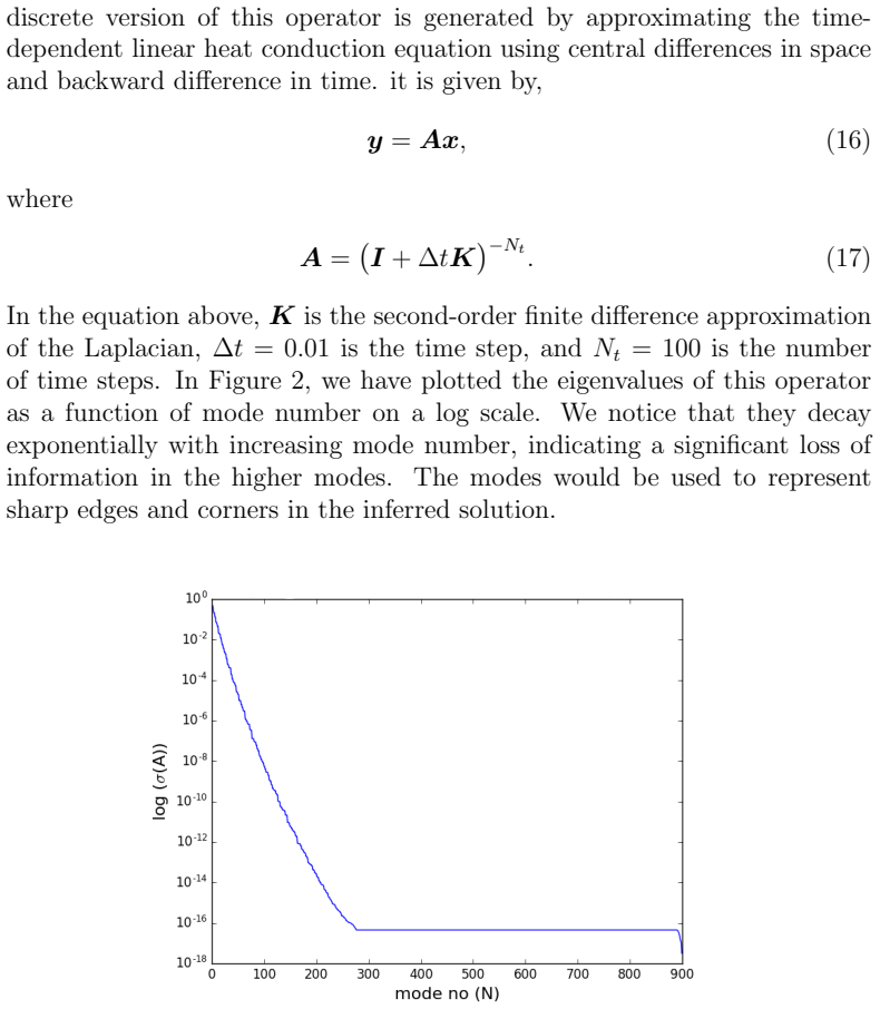
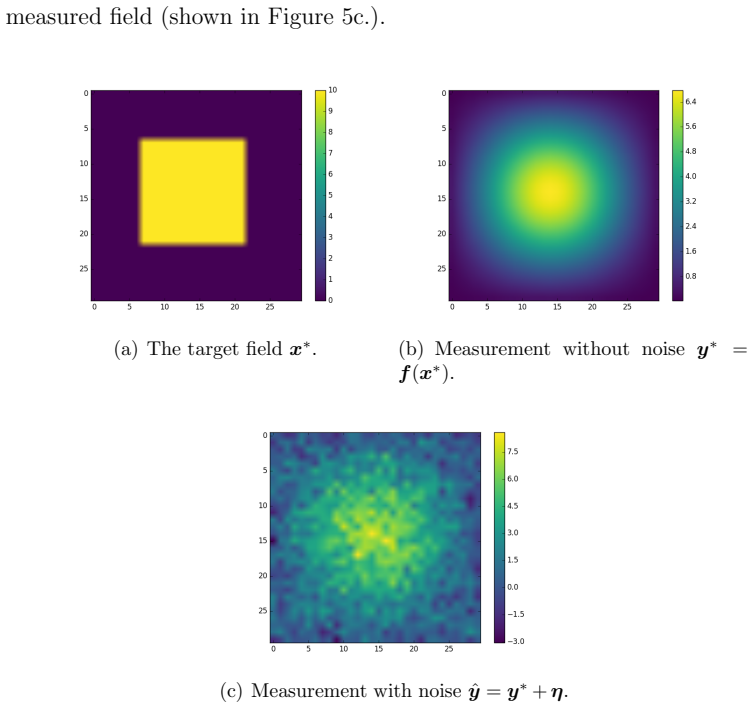
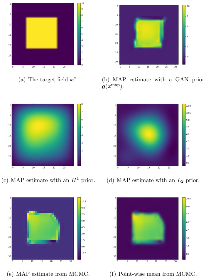
The paper shows that once a GAN is trained on samples of a field, its generator can be used directly as the prior in a Bayesian inference procedure. This approximates the distribution of the field of interest and allows the update to be performed even when the field has a large discrete dimension and the prior is complex, as illustrated in the heat conduction example where the initial temperature is inferred from later noisy temperature data.
What carries the argument
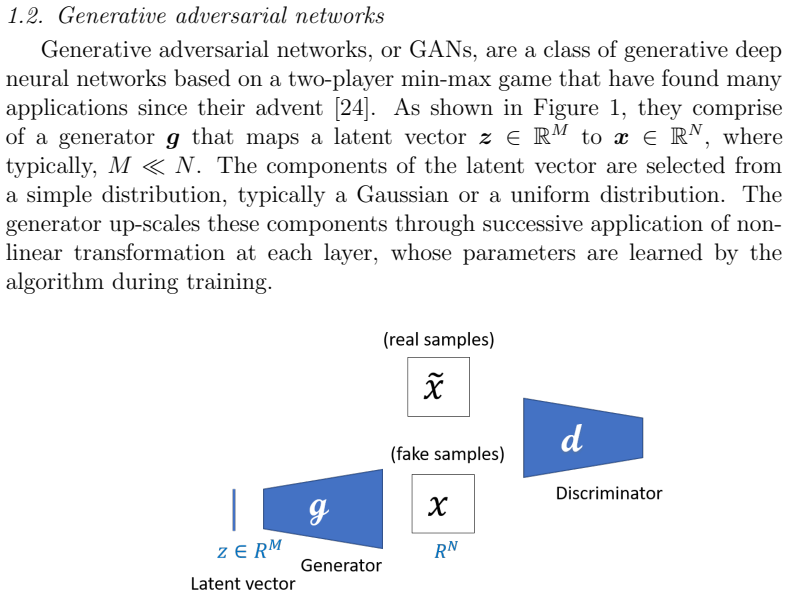
The GAN generator, which maps the components of a low-dimensional latent vector to an approximation of the distribution of the high-dimensional field of interest, serving as the prior in the Bayesian update.
Load-bearing premise
The samples generated by the trained GAN are distributed closely enough to the true prior that the Bayesian posterior computed with them remains a good approximation to the true posterior.
What would settle it
Compare the posterior mean and variance obtained using the GAN prior against those from an exact Bayesian update on a test problem where the true prior distribution is known and easy to sample from.
Figures
read the original abstract
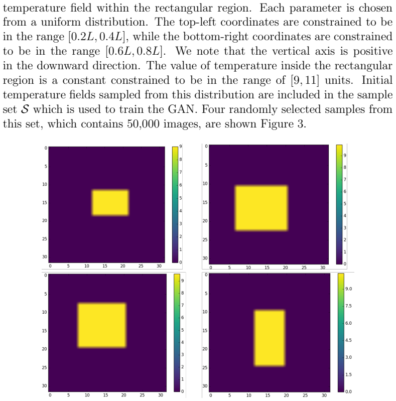
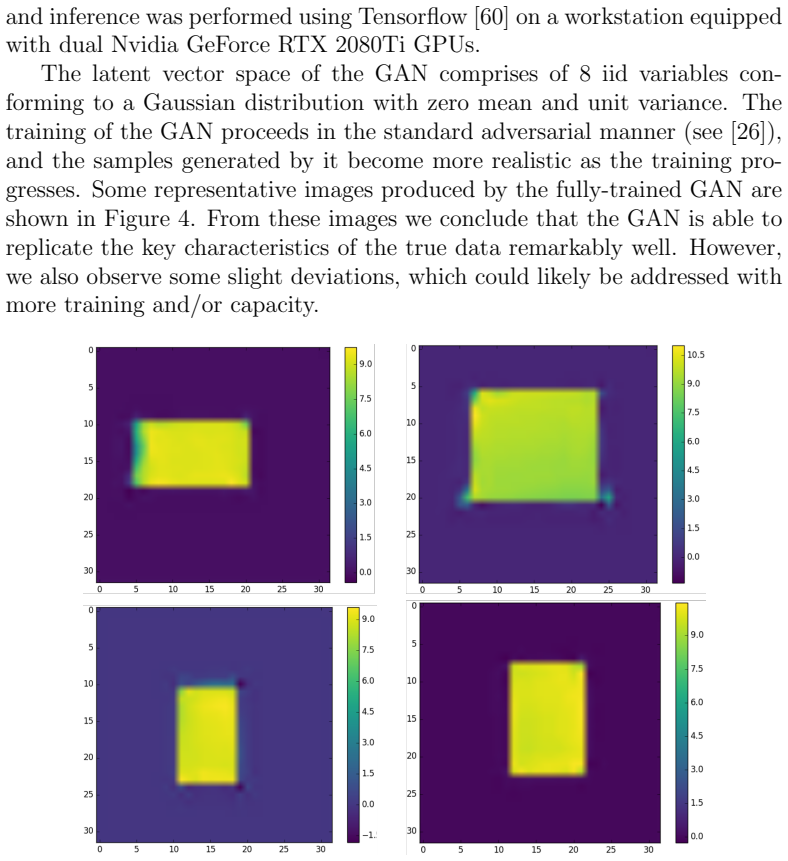
Bayesian inference is used extensively to infer and to quantify the uncertainty in a field of interest from a measurement of a related field when the two are linked by a physical model. Despite its many applications, Bayesian inference faces challenges when inferring fields that have discrete representations of large dimension, and/or have prior distributions that are difficult to represent mathematically. In this manuscript we consider the use of Generative Adversarial Networks (GANs) in addressing these challenges. A GAN is a type of deep neural network equipped with the ability to learn the distribution implied by multiple samples of a given field. Once trained on these samples, the generator component of a GAN maps the iid components of a low-dimensional latent vector to an approximation of the distribution of the field of interest. In this work we demonstrate how this approximate distribution may be used as a prior in a Bayesian update, and how it addresses the challenges associated with characterizing complex prior distributions and the large dimension of the inferred field. We demonstrate the efficacy of this approach by applying it to the problem of inferring and quantifying uncertainty in the initial temperature field in a heat conduction problem from a noisy measurement of the temperature at later time.
Editorial analysis
A structured set of objections, weighed in public.
Referee Report
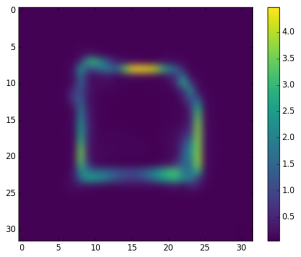
Summary. The manuscript proposes using a trained GAN generator as an approximate prior for Bayesian inference on high-dimensional fields with complex distributions. The generator maps low-dimensional latent vectors to field samples; Bayesian updating is performed via MCMC sampling in latent space. The approach is demonstrated on inferring the initial temperature field in a 1D heat conduction problem from noisy temperature measurements at a later time, yielding plausible posterior fields and uncertainty estimates.
Significance. If the GAN distribution is sufficiently close to the true prior, the method addresses a practical barrier in Bayesian inference by replacing hand-specified priors with data-driven ones while reducing the effective dimension of the sampling problem. The use of standard MCMC in latent space (rather than custom samplers) and the reporting of plausible posterior fields are concrete strengths that support feasibility for similar inverse problems.
minor comments (3)
- The abstract states that the GAN 'addresses the challenges associated with characterizing complex prior distributions,' but the manuscript should explicitly note (e.g., in the discussion or conclusions) that this holds only to the extent that the trained generator matches the empirical distribution of the training samples; no quantitative distance metric between GAN samples and held-out prior samples is reported.
- Notation for the latent-space posterior (p(z | data)) versus the induced field posterior should be clarified in §3 or §4 to avoid ambiguity when the generator is non-invertible.
- Figure captions for the heat-conduction results should include the number of MCMC samples retained after burn-in and the acceptance rate, as these directly affect the reliability of the reported posterior means and variances.
Simulated Author's Rebuttal
We thank the referee for the positive summary of our work and the recommendation of minor revision. No specific major comments were raised in the report.
Circularity Check
No significant circularity identified
full rationale
The manuscript trains a GAN generator on external samples to approximate a complex high-dimensional prior, then performs standard MCMC sampling in the latent space of that fixed generator to obtain the posterior. No equation in the provided text defines a quantity in terms of itself, renames a fitted parameter as a prediction, or relies on a self-citation chain for a uniqueness claim. The Bayesian update step uses the trained generator as an external black-box map; the heat-conduction demonstration reports posterior statistics without claiming that any derived quantity is forced by the training data alone. The derivation chain therefore remains independent of its own inputs.
Axiom & Free-Parameter Ledger
free parameters (1)
- GAN latent dimension
axioms (2)
- domain assumption A GAN trained on samples can approximate the distribution of the field of interest sufficiently well for use as a prior.
- standard math Standard Bayesian update remains valid when the prior is replaced by samples from a generator network.
Lean theorems connected to this paper
-
IndisputableMonolith/Cost/FunctionalEquation.leanwashburn_uniqueness_aczel unclear?
unclearRelation between the paper passage and the cited Recognition theorem.
the generator component of a GAN maps the iid components of a low-dimensional latent vector to an approximation of the distribution of the field of interest... sampling from the posterior distribution for x is equivalent to sampling from the posterior distribution for z
-
IndisputableMonolith/Foundation/RealityFromDistinction.leanreality_from_one_distinction unclear?
unclearRelation between the paper passage and the cited Recognition theorem.
Wasserstein GAN... minimizes the Wasserstein metric between ptrue_X(x) and pgen_X(x)
What do these tags mean?
- matches
- The paper's claim is directly supported by a theorem in the formal canon.
- supports
- The theorem supports part of the paper's argument, but the paper may add assumptions or extra steps.
- extends
- The paper goes beyond the formal theorem; the theorem is a base layer rather than the whole result.
- uses
- The paper appears to rely on the theorem as machinery.
- contradicts
- The paper's claim conflicts with a theorem or certificate in the canon.
- unclear
- Pith found a possible connection, but the passage is too broad, indirect, or ambiguous to say the theorem truly supports the claim.
Reference graph
Works this paper leans on
- [1]
- [2]
- [3]
-
[4]
W. P. Gouveia, J. A. Scales, Resolution of seismic waveform inversion: Bayes versus Occam, Inverse Problems 13 (1997) 323–349
work page 1997
-
[5]
A. Malinverno, Parsimonious Bayesian Markov chain Monte Carlo in- version in a nonlinear geophysical problem, Geophysical Journal Inter- national 151 (2002) 675–688
work page 2002
- [6]
-
[7]
T. Isaac, N. Petra, G. Stadler, O. Ghattas, Scalable and efficient algo- rithms for the propagation of uncertainty from data through inference to prediction for large-scale problems, with application to flow of the 20 Antarctic ice sheet, Journal of Computational Physics 296 (2015) 348– 368
work page 2015
-
[8]
C. Jackson, M. K. Sen, P. L. Stoffa, C. Jackson, M. K. Sen, P. L. Stoffa, An Efficient Stochastic Bayesian Approach to Optimal Parameter and Uncertainty Estimation for Climate Model Predictions, Journal of Cli- mate 17 (2004) 2828–2841
work page 2004
-
[9]
H. N. Najm, B. J. Debusschere, Y. M. Marzouk, S. Widmer, O. P. Le Ma ˜A R⃝tre, Uncertainty quantification in chemical systems, Interna- tional Journal for Numerical Methods in Engineering 80 (2009) 789–814
work page 2009
-
[10]
J. Wang, N. Zabaras, Hierarchical bayesian models for inverse problems in heat conduction, Inverse Problems 21 (2004) 183–206
work page 2004
-
[11]
T. J. Loredo, From Laplace to Supernova SN 1987A: Bayesian Inference in Astrophysics, in: Maximum Entropy and Bayesian Methods, Springer Netherlands, Dordrecht, 1990, pp. 81–142
work page 1990
-
[12]
A. Asensio Ramos, M. J. Mart´ ınez Gonz´ alez, J. A. Rubi˜ no-Mart´ ın, Bayesian inversion of Stokes profiles, Astronomy & Astrophysics 476 (2007) 959–970
work page 2007
-
[13]
T. J. Sabin, C. A. L. Bailer-Jones, P. J. Withers, Accelerated learning using Gaussian process models to predict static recrystallization in an Al-Mg alloy, Modelling and Simulation in Materials Science and Engi- neering 8 (2000) 687–706
work page 2000
-
[14]
S. Siltanen, V. Kolehmainen, S. J rvenp, J. P. Kaipio, P. Koistinen, M. Lassas, J. Pirttil, E. Somersalo, Statistical inversion for medical x- ray tomography with few radiographs: I. General theory, Physics in Medicine and Biology 48 (2003) 1437–1463
work page 2003
-
[15]
V. Kolehmainen, A. Vanne, S. Siltanen, S. Jarvenpaa, J. Kaipio, M. Las- sas, M. Kalke, Parallelized Bayesian inversion for three-dimensional den- tal X-ray imaging, IEEE Transactions on Medical Imaging 25 (2006) 218–228
work page 2006
-
[16]
Tarantola, Inverse problem theory and methods for model parameter estimation, volume 89, siam, 2005
A. Tarantola, Inverse problem theory and methods for model parameter estimation, volume 89, siam, 2005. 21
work page 2005
-
[17]
L. Fahrmeir, S. Lang, Bayesian inference for generalized additive mixed models based on Markov random field priors, Journal of the Royal Statistical Society: Series C (Applied Statistics) 50 (2001) 201–220
work page 2001
-
[18]
A. M. Stuart, Inverse problems: A Bayesian perspective, Acta Numerica 19 (2010) 451–559
work page 2010
-
[19]
Y. M. Marzouk, H. N. Najm, Dimensionality reduction and polynomial chaos acceleration of Bayesian inference in inverse problems, Journal of Computational Physics 228 (2009) 1862–1902
work page 2009
-
[20]
D. Calvetti, E. Somersalo, Hypermodels in the Bayesian imaging frame- work, Inverse Problems 24 (2008) 034013
work page 2008
-
[21]
T. Bui-Thanh, C. Burstedde, O. Ghattas, J. Martin, G. Stadler, L. C. Wilcox, Extreme-scale UQ for Bayesian inverse problems governed by PDEs, in: 2012 International Conference for High Performance Com- puting, Networking, Storage and Analysis, IEEE, 2012, pp. 1–11
work page 2012
-
[22]
C. Han, B. P. Carlin, Markov chain monte carlo methods for computing bayes factors: A comparative review, Journal of the American Statistical Association 96 (2001) 1122–1132
work page 2001
-
[23]
M. D. Parno, Y. M. Marzouk, Transport map accelerated markov chain monte carlo, SIAM/ASA Journal on Uncertainty Quantification 6 (2018) 645–682
work page 2018
-
[24]
I. Goodfellow, J. Pouget-Abadie, M. Mirza, B. Xu, D. Warde-Farley, S. Ozair, A. Courville, Y. Bengio, Generative adversarial nets, in: Advances in neural information processing systems, pp. 2672–2680
- [25]
-
[26]
I. Gulrajani, F. Ahmed, M. Arjovsky, V. Dumoulin, A. C. Courville, Im- proved training of wasserstein gans, in: Advances in neural information processing systems, pp. 5767–5777
-
[27]
A. Makhzani, J. Shlens, N. Jaitly, I. Goodfellow, B. Frey, Adversarial Autoencoders (2015)
work page 2015
-
[28]
V. Dumoulin, I. Belghazi, B. Poole, O. Mastropietro, A. Lamb, M. Ar- jovsky, A. Courville, Adversarially Learned Inference (2016). 22
work page 2016
-
[29]
L. Mescheder, S. Nowozin, A. Geiger, Adversarial Variational Bayes: Unifying Variational Autoencoders and Generative Adversarial Net- works (2017)
work page 2017
- [30]
- [31]
-
[32]
MaskGAN: Better Text Generation via Filling in the______
W. Fedus, I. Goodfellow, A. M. Dai, Maskgan: better text generation via filling in the , arXiv preprint arXiv:1801.07736 (2018)
work page internal anchor Pith review Pith/arXiv arXiv 2018
-
[33]
S. Tulyakov, M.-Y. Liu, X. Yang, J. Kautz, Mocogan: Decomposing motion and content for video generation, in: Proceedings of the IEEE conference on computer vision and pattern recognition, pp. 1526–1535
-
[34]
L. Ma, X. Jia, Q. Sun, B. Schiele, T. Tuytelaars, L. Van Gool, Pose Guided Person Image Generation (2017)
work page 2017
-
[35]
T.-C. Wang, M.-Y. Liu, J.-Y. Zhu, A. Tao, J. Kautz, B. Catanzaro, High-Resolution Image Synthesis and Semantic Manipulation with Con- ditional GANs (2017)
work page 2017
-
[36]
M. Vauhkonen, J. P. Kaipio, E. Somersalo, P. A. Karjalainen, Electri- cal impedance tomography with basis constraints, Inverse Problems 13 (1997) 523–530
work page 1997
-
[37]
D. Calvetti, E. Somersalo, Priorconditioners for linear systems, Inverse Problems 21 (2005) 1397–1418
work page 2005
-
[38]
C. Lieberman, K. Willcox, O. Ghattas, Parameter and State Model Reduction for Large-Scale Statistical Inverse Problems, SIAM Journal on Scientific Computing 32 (2010) 2523–2542
work page 2010
- [39]
-
[40]
K. H. Jin, M. T. McCann, E. Froustey, M. Unser, Deep Convolutional Neural Network for Inverse Problems in Imaging, IEEE Transactions on Image Processing 26 (2017) 4509–4522. 23
work page 2017
- [41]
-
[42]
J. H. R. Chang, C.-L. Li, B. Barnab´ as, P. . Oczos, B. V. K. V. Kumar, A. C. Sankaranarayanan, One Network to Solve Them All-Solving Linear Inverse Problems using Deep Projection Models, Technical Report, ????
- [43]
-
[44]
Q. Yang, P. Yan, Y. Zhang, H. Yu, Y. Shi, X. Mou, M. K. Kalra, Y. Zhang, L. Sun, G. Wang, Low-Dose CT Image Denoising Using a Generative Adversarial Network With Wasserstein Distance and Percep- tual Loss, IEEE Transactions on Medical Imaging 37 (2018) 1348–1357
work page 2018
- [45]
-
[46]
R. Anirudh, J. J. Thiagarajan, B. Kailkhura, T. Bremer, An Unsuper- vised Approach to Solving Inverse Problems using Generative Adversar- ial Networks (2018)
work page 2018
-
[47]
P. Isola, J.-Y. Zhu, T. Zhou, A. A. Efros, Image-to-image translation with conditional adversarial networks, arxiv (2016)
work page 2016
-
[48]
J.-Y. Zhu, T. Park, P. Isola, A. A. Efros, Unpaired image-to-image translation using cycle-consistent adversarial networks, in: Computer Vision (ICCV), 2017 IEEE International Conference on
work page 2017
-
[49]
T. Kim, M. Cha, H. Kim, J. K. Lee, J. Kim, Learning to Discover Cross-Domain Relations with Generative Adversarial Networks (2017)
work page 2017
-
[50]
S. Lunz, O. ¨Oktem, C.-B. Sch¨ onlieb, Adversarial regularizers in inverse problems, in: Advances in Neural Information Processing Systems, pp. 8507–8516. 24
-
[51]
A. Bora, A. Jalal, E. Price, A. G. Dimakis, Compressed sensing using generative models, in: Proceedings of the 34th International Conference on Machine Learning-Volume 70, JMLR. org, pp. 537–546
-
[52]
A. Bora, E. Price, A. G. Dimakis, Ambientgan: Generative models from lossy measurements., ICLR 2 (2018) 5
work page 2018
- [53]
-
[54]
Y. Wu, M. Rosca, T. Lillicrap, Deep compressed sensing, arXiv preprint arXiv:1905.06723 (2019)
work page internal anchor Pith review Pith/arXiv arXiv 1905
-
[55]
V. Shah, C. Hegde, Solving linear inverse problems using gan priors: An algorithm with provable guarantees, in: 2018 IEEE International Con- ference on Acoustics, Speech and Signal Processing (ICASSP), IEEE, pp. 4609–4613
work page 2018
- [56]
-
[57]
Gal, Uncertainty in deep learning, Ph.D
Y. Gal, Uncertainty in deep learning, Ph.D. thesis, PhD thesis, Univer- sity of Cambridge, 2016
work page 2016
-
[58]
Y. Gal, Z. Ghahramani, Dropout as a Bayesian Approximation: Repre- senting Model Uncertainty in Deep Learning (2015)
work page 2015
-
[59]
K. He, X. Zhang, S. Ren, J. Sun, Deep Residual Learning for Image Recognition (2015)
work page 2015
-
[60]
M. Abadi, A. Agarwal, P. Barham, E. Brevdo, Z. Chen, C. Citro, G. S. Corrado, A. Davis, J. Dean, M. Devin, S. Ghemawat, I. Goodfellow, A. Harp, G. Irving, M. Isard, Y. Jia, R. Jozefowicz, L. Kaiser, M. Kud- lur, J. Levenberg, D. Man´ e, R. Monga, S. Moore, D. Murray, C. Olah, M. Schuster, J. Shlens, B. Steiner, I. Sutskever, K. Talwar, P. Tucker, V. Vanho...
work page 2015
-
[61]
N. Metropolis, A. W. Rosenbluth, M. N. Rosenbluth, A. H. Teller, E. Teller, Equation of State Calculations by Fast Computing Machines, The Journal of Chemical Physics 21 (1953) 1087–1092
work page 1953
-
[62]
W. K. Hastings, Monte Carlo Sampling Methods Using Markov Chains and Their Applications, Biometrika 57 (1970) 97
work page 1970
-
[63]
Y. F. Atchad´ e, An Adaptive Version for the Metropolis Adjusted Langevin Algorithm with a Truncated Drift, Methodology and Com- puting in Applied Probability 8 (2006) 235–254
work page 2006
-
[64]
M. D. Hoffman, A. Gelman, The No-U-Turn Sampler: Adaptively Set- ting Path Lengths in Hamiltonian Monte Carlo, Technical Report, 2014
work page 2014
-
[65]
S. Brooks, A. Gelman, G. Jones, X.-L. Meng, R. M. Neal, MCMC using Hamiltonian dynamics, Technical Report, 2012. 26 Appendix A. Architecture details The architecture of the generator component of the GAN is shown in Figure A.8, and the architecture of the discriminator is shown in Figure A.9. Some notes regarding the nomenclature used in these figures: • C...
work page 2012
discussion (0)
Sign in with ORCID, Apple, or X to comment. Anyone can read and Pith papers without signing in.