REVIEW 4 major objections 6 minor 77 references
Dual-Branch Subpixel-Guided Network for Hyperspectral Image Classification
T0 review · 4 major / 6 minor · reviewed 2026-08-11 · deepseek-v4-flash
Pith's one-line read A dual-branch network that fuses autoencoder-derived subpixel abundances with convolutional class features achieves top accuracy on three hyperspectral benchmarks.
desk verdict DSNet is a legit multi-task architecture with solid experiments, but the 'unsupervised subpixel guidance' claim is confounded by CE gradients flowing into the unmixing encoder. read the letter →
The pith
A machine-rendered reading of the paper's core claim, the machinery that carries it, and where it could break.
The reading
What carries the argument
The engine of the method is the deep autoencoder unmixing branch, whose general mixing decoder implements the model $Y = MA + \Phi(MA) + N$, combining a linear mixture term with a nonlinear fluctuation term through a single trainable weight matrix $G$ that makes the decoder insensitive to the number of layers. The encoder produces abundance maps $\mathbf{v}_i$ with enforced abundance non-negativity and sum-to-one constraints using absolute-value rectification and summed normalization. A subpixel fusion module reduces the spatial dimension of the abundance patch with a stride-2 convolution, flattens it, and concatenates it with the pixel-level class feature from a two-layer 2D CNN branch; a linear layer converts the joint representation into class predictions. The network is trained end-to-end with the objective $\mathcal{L} = \lambda \mathcal{L}_{\mathrm{RE}} + (1-\lambda)\mathcal{L}_{\mathrm{CE}}$, where $\mathcal{L}_{\mathrm{RE}}$ is the spectral angle distance between the reconstructed and input patches and $\mathcal{L}_{\mathrm{CE}}$ is the cross-entropy classification loss.
What would settle it
A concrete test: run DSNet with the unmixing branch's encoder replaced by a randomly initialized, fixed feature extractor of the same architecture. If the classification gain over the CNN-only baseline persists, the improvement cannot be attributed to learned subpixel information; alternatively, compare the learned abundance maps against known reference abundances on synthetic mixed-pixel scenes, where ground-truth fractions are available, to check whether the abundances are physically correct.
Extended reading notes
Core claim
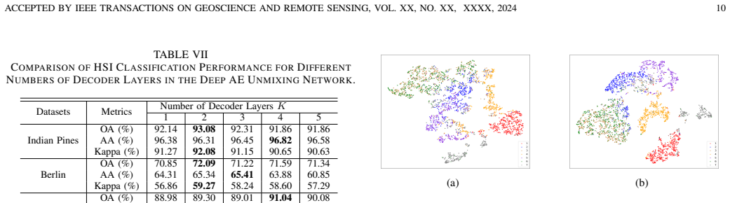
The central claim is that automatically integrating subpixel unmixing information with convolutional class features improves hyperspectral image classification. The deep autoencoder unmixing branch encodes each input patch into abundance maps that satisfy non-negativity and sum-to-one constraints and decodes them through a general mixing model that combines a linear mixture with a physically motivated nonlinear fluctuation term. A subpixel fusion module concatenates the spatial-reduced abundance maps with the CNN branch's class features before a final linear classifier, and the whole network is trained with a weighted sum of spectral-angle reconstruction loss and cross-entropy loss. In the reported experiments DSNet achieves the highest overall accuracy and Kappa on all three datasets, with best overall accuracy, average accuracy, and Kappa of 93.08%, 96.31%, and 92.08% on Indian Pines and corresponding leading marks on Berlin (72.09% OA, 59.27% Kappa) and Augsburg (89.30% OA, 84.62% Kappa). Ablation studies show that both the nonlinear decoder and the fusion module contribute to the gain, and the paper therefore claims that subpixel guidance yields more reliable decision boundaries and better class separation than pixel-level features alone.
Load-bearing premise
The load-bearing premise is that the abundance maps learned by the autoencoder, trained only to reconstruct spectra, genuinely contain subpixel mixing information that helps the classifier; the paper explicitly declines to validate the unmixing results quantitatively.
Editorial extensions
If this is right
- On the Indian Pines, Berlin, and Augsburg datasets, DSNet attains the highest overall accuracy and Kappa among all compared methods, and the highest average accuracy on Indian Pines and Augsburg.
- Ablation experiments show the nonlinear decoder adds roughly 1.1 to 1.3 percentage points of overall accuracy over the linear decoder, and the subpixel fusion module adds another 1.3 to 2.1 points, indicating both components carry weight.
- Per-epoch training time stays below the 3D CNN, GRU, ViT, MorphConv, and SSFTT baselines on all three datasets, so the dual-branch design does not come at prohibitive computational cost.
- With training ratios at or below 20%, DSNet's accuracy drops below some hybrid baselines, suggesting the unsupervised unmixing branch needs a minimum amount of data to produce stable abundance estimates.
Reading between the lines
- The paper does not quantitatively evaluate the estimated abundances; a direct test would compare DSNet's abundance maps against reference abundances on synthetic mixed-pixel data, or replace the trained unmixing branch with a random untrained encoder to see whether the accuracy gain persists. If the gain does persist, the benefit may come from added model capacity rather than subpixel information.
- The optimal fusion weight $\lambda$ differs across datasets (0.2, 0.8, 0.1), so a learned or adaptive weighting scheme could improve robustness and reduce per-dataset tuning.
- The same dual-branch recipe could transfer to other per-pixel remote sensing tasks, such as target detection or land-cover mapping from low-resolution satellite imagery where mixed pixels are common.
- Because the unmixing branch saturates at low training ratios, pretraining it on unlabeled pixels or on a larger auxiliary scene could lower the data requirement for the joint classifier.
Editorial analysis
A structured set of objections, weighed in public.
Referee Report
Summary. The manuscript proposes DSNet, a dual-branch network for hyperspectral image classification. One branch is a deep autoencoder unmixing network with a general mixing decoder that estimates abundance maps; the other is a simple 2D CNN that extracts pixel-level class features. A subpixel fusion module concatenates a spatially transformed abundance representation with the class feature, and a linear classifier produces the prediction. Training minimizes a weighted sum of a spectral angle distance reconstruction loss and a cross-entropy classification loss. Experiments on Indian Pines, Berlin, and Augsburg report OA/AA/Kappa, per-class accuracy, training time, training-ratio curves, ablations, decoder-layer counts, the fusion weight λ, t-SNE plots, and abundance-map visualizations. The paper claims that DSNet achieves the highest classification accuracy on all three datasets and that the improvement is due to integrating unsupervised subpixel abundance information.
Significance. The motivating idea is useful: rather than treating every pixel as pure, a physically motivated mixing model could provide complementary subpixel information for classification. The experimental effort is substantial, with three datasets, seven comparison methods, ablations, computational cost comparisons, and code availability. However, the central causal claim is currently not established. As described in Section II-C, the cross-entropy loss backpropagates through the fusion module into the unmixing encoder, so the abundances are not trained in an unsupervised manner, contrary to the abstract's claim. The λ=0 experiment in Fig. 7 is not a true ablation of the unmixing branch, and Section III-D3 explicitly declines quantitative validation of the abundances. The accuracy gains in Table VI could therefore come from added capacity, the reconstruction regularizer, or class-supervised shaping of the encoder rather than from diagnostic subpixel information. The comparisons also lack error bars and significance testing. With additional controlled experiments, the contribution could be a valuable one, but the evidence in the current version does not support the mechanism claimed.
major comments (4)
- [§II-C, Eqs. (14)-(18); §III-D3] The classification loss L_CE is applied to p̂_i = W_out s_i, where s_i contains v_i, the encoder output of the unmixing branch. Consequently, CE gradients flow into the unmixing encoder through the fusion module, so the abundance maps are not extracted in an "unsupervised manner" as claimed in the Abstract and Section II-B1. The paper itself acknowledges this in Section III-D3, where the abundance maps are said to be "optimized from the perspective of both deep AE unmixing and CNN-based classifier network." This makes the ablation gains in Table VI (e.g., +3.88% OA on Indian Pines for the full model over the nonlinear-decoder-only variant) uninterpretable as evidence for the value of subpixel information. The authors should re-run the ablations with the abundance path detached from L_CE (e.g., stop-gradient on v_i before the fusion module, or training the unmixing branch in a separate phase with frozen weights) and report whether the accuracy gains persist.
- [§III-D2, Fig. 7] The statement "When λ is set to 0, it means that unmixing part has no effect" is incorrect. Setting λ=0 only removes the reconstruction loss L_RE; the unmixing encoder still receives gradients from L_CE through the fusion path, so the branch still influences the classifier. Fig. 7 therefore cannot be used to conclude that the unmixing part contributes nothing at λ=0 or that the performance increase with larger λ is due to subpixel information alone. A true disable condition would remove the fusion connection or freeze the unmixing encoder, and the corresponding curves should be reported.
- [Tables II-IV and Table VI] All quantitative results are reported as single runs without variance or significance tests. Several decisive differences are small, for example 89.30% vs. 87.66% OA on Augsburg and differences of about 1% between ablation configurations, and these could be within run-to-run variability. The authors should report mean and standard deviation over multiple random seeds for all methods and ablations, and where possible perform a significance test (e.g., McNemar's test or paired evaluation) to support the claim that DSNet is statistically superior.
- [§III-D3] The authors explicitly decline to validate the unmixing results quantitatively, and the abundance visualizations in Fig. 9 are not sufficient to show that the extracted maps encode genuine subpixel mixing information. The central claim would be substantially strengthened by a synthetic-data experiment with known endmembers and abundances, reporting abundance error or endmember SAD, or by a control network with the same architecture and capacity but without the reconstruction constraint. Without such evidence, the physical "subpixel" interpretation remains an untested assumption, and the classification gains could be a generic effect of the extra branch.
minor comments (6)
- [Eq. (9)] The index i is used both for the pixel/position index and as the summation index over abundance components; using a different dummy index (e.g., j) would make the normalization over the P abundance channels unambiguous.
- [§II-B1, Table I] The intermediate encoder dimensions are not clearly stated in the text. Table I lists L/2, L/4, and P for the three encoder blocks, but Eq. (8) writes h_i^(e) ∈ R^{P×H×H} for all layers; the text should clarify the channel dimensions at each layer.
- [Fig. 7] The three curves in Fig. 7 are not identified by a legend or distinct markers in the text description, making it difficult to associate each curve with Indian Pines, Berlin, and Augsburg. Adding a legend would improve readability.
- [I, Introduction] There are minor typos: "have be proposed" should be "have been proposed," and "urban planing" should be "urban planning."
- [Table I] The table mixes the unmixing decoder, the classifier output, and the fusion module in the same "Block 4/5" columns, which is confusing. Reformating the table so that the decoder and classifier paths are visually separated would help the reader follow the architecture.
- [Fig. 9] The abundance maps in Fig. 9 lack a color scale and axis labels; adding a colorbar and specifying which abundance/endmember each map corresponds to would make the visualization informative.
Circularity Check
No circular derivation: DSNet's accuracy is externally benchmarked; the main issues are unsupported causal attribution and non-load-bearing self-citations, not circularity.
full rationale
The central performance claim (Section III-B) is tested on held-out test pixels with fixed splits shared by all methods (Tables II-IV), so the reported OA/AA/Kappa are external evidence rather than quantities reconstructed from the training objective. The 'unsupervised' claim is undermined by the paper's own equations: in Eq. (18), L = λL_RE + (1−λ)L_CE, and L_CE reaches the AE encoder through the fusion module (Eqs. 14-15), so CE supervises the 'abundance' branch; similarly, the statement that λ=0 means 'unmixing part has no effect' is not implied by the equations. These are confounds for the causal attribution of gains to subpixel content, not reductions of a prediction to its inputs. Section III-D3 explicitly declines to validate the abundances quantitatively, which further weakens the physical interpretation but again is a validity limitation. The prior unmixing self-citations (refs [59], [62]-[64]) are background and motivation; the decoder construction (Eqs. 10-12) is made in-paper and no load-bearing claim rests on an unverified self-cited theorem. Therefore no specific circular step can be exhibited, and the score reflects only minor, non-load-bearing self-citation.
Assumptions & free parameters
free parameters (4)
- fusion coefficient λ =
0.5 (fixed after tuning; per-dataset best: 0.2, 0.8, 0.1)
- number of decoder layers K =
2 (fixed after tuning, range 1-5 tested)
- patch size =
7x7 (Indian Pines, Augsburg), 5x5 (Berlin)
- learning rate schedule =
1e-3, decay 0.9 per 50 epochs
assumptions (3)
- domain assumption Spectral mixing is described by LMM plus a nonlinear fluctuation term (Eq. 5)
- domain assumption 1x1 convolution is equivalent to a fully connected layer for spectral unmixing
- ad hoc to paper The extracted abundance maps are meaningful for classification
Cite this review
Pith. "Pith review of Dual-Branch Subpixel-Guided Network for Hyperspectral Image Classification." pith.science (2026). https://pith.science/paper/2BCMPNNR
@misc{pith2026241203893,
  author       = {Pith},
  title        = {Pith review of: Dual-Branch Subpixel-Guided Network for Hyperspectral Image Classification},
  year         = {2026},
  howpublished = {\url{https://pith.science/paper/2BCMPNNR}},
  note         = {Machine review of arXiv:2412.03893}
}
read the original abstract
Deep learning (DL) has been widely applied into hyperspectral image (HSI) classification owing to its promising feature learning and representation capabilities. However, limited by the spatial resolution of sensors, existing DL-based classification approaches mainly focus on pixel-level spectral and spatial information extraction through complex network architecture design, while ignoring the existence of mixed pixels in actual scenarios. To tackle this difficulty, we propose a novel dual-branch subpixel-guided network for HSI classification, called DSNet, which automatically integrates subpixel information and convolutional class features by introducing a deep autoencoder unmixing architecture to enhance classification performance. DSNet is capable of fully considering physically nonlinear properties within subpixels and adaptively generating diagnostic abundances in an unsupervised manner to achieve more reliable decision boundaries for class label distributions. The subpixel fusion module is designed to ensure high-quality information fusion across pixel and subpixel features, further promoting stable joint classification. Experimental results on three benchmark datasets demonstrate the effectiveness and superiority of DSNet compared with state-of-the-art DL-based HSI classification approaches. The codes will be available at https://github.com/hanzhu97702/DSNet, contributing to the remote sensing community.
Figures


Figures from the paper (5 more)



Reference graph
Works this paper leans on
-
[1]
Hyperspectral remote sensing data analysis and future challenges,
J. M. Bioucas-Dias, A. Plaza, G. Camps-Valls, P. Scheunders, N. Nasrabadi, and J. Chanussot, “Hyperspectral remote sensing data analysis and future challenges,” IEEE Geosci. Remote Sens. Mag., vol. 1, no. 2, pp. 6–36, Jun. 2013
work page 2013
-
[2]
L. He, J. Li, C. Liu, and S. Li, “Recent advances on spectral–spatial hyperspectral image classification: An overview and new guidelines,” IEEE Trans. Geosci. Remote Sens., vol. 56, no. 3, pp. 1579–1597, 2018
work page 2018
-
[3]
Eigen-cnn: Eigenimages plus eigennoise level maps guided network for hyperspectral image denoising,
L. Zhuang, M. K. Ng, L. Gao, and Z. Wang, “Eigen-cnn: Eigenimages plus eigennoise level maps guided network for hyperspectral image denoising,” IEEE Trans. Geosci. Remote Sens. , pp. 1–18, 2024
work page 2024
-
[4]
P. C. Pandey, P. K. Srivastava, H. Balzter, B. Bhattacharya, and G. P. Petropoulos, “8 - hyperspectral remote sensing in precision agriculture: present status, challenges, and future trends,” in Hyperspectral Remote Sens. Elsevier, 2020, pp. 121–146
work page 2020
-
[5]
D. Haboudane, J. R. Miller, E. Pattey, P. J. Zarco-Tejada, and I. B. Strachan, “Hyperspectral vegetation indices and novel algorithms for predicting green lai of crop canopies: Modeling and validation in the context of precision agriculture,” Remote Sens. Environ., vol. 90, no. 3, pp. 337–352, 2004
work page 2004
-
[6]
Understanding urban landuse from the above and ground perspectives: A deep learning, multimodal solution,
S. Srivastava, J. E. Vargas-Munoz, and D. Tuia, “Understanding urban landuse from the above and ground perspectives: A deep learning, multimodal solution,” Remote Sens. Environ. , vol. 228, pp. 129–143, 2019
2019
-
[7]
Local climate zone-based urban land cover classification from multi-seasonal sentinel-2 images with a recurrent residual network,
C. Qiu, L. Mou, M. Schmitt, and X. X. Zhu, “Local climate zone-based urban land cover classification from multi-seasonal sentinel-2 images with a recurrent residual network,” ISPRS J. Photogramm. Remote Sens., vol. 154, pp. 151–162, 2019
2019
-
[8]
Bs3lnet: A new blind-spot self-supervised learning network for hyperspectral anomaly detection,
L. Gao, D. Wang, L. Zhuang, X. Sun, M. Huang, and A. Plaza, “Bs3lnet: A new blind-spot self-supervised learning network for hyperspectral anomaly detection,” IEEE Trans. Geosci. Remote Sens. , vol. 61, pp. 1–18, 2023
work page 2023
Show all 77 references
-
[9]
Hadgsm: A unified nonconvex framework for hyperspectral anomaly detection,
L. Ren, L. Gao, M. Wang, X. Sun, and J. Chanussot, “Hadgsm: A unified nonconvex framework for hyperspectral anomaly detection,” IEEE Trans. Geosci. Remote Sens. , vol. 62, pp. 1–15, 2024
2024
-
[10]
Comparison of airborne hyperspectral data and eo-1 hyperion for mineral mapping,
F. Kruse, J. Boardman, and J. Huntington, “Comparison of airborne hyperspectral data and eo-1 hyperion for mineral mapping,” IEEE Trans. Geosci. Remote Sens. , vol. 41, no. 6, pp. 1388–1400, 2003
2003
-
[11]
Hyperspectral remote sensing in litho- logical mapping, mineral exploration, and environmental geology: an updated review,
S. Peyghambari and Y . Zhang, “Hyperspectral remote sensing in litho- logical mapping, mineral exploration, and environmental geology: an updated review,” J. Appl. Remote Sens. , vol. 15, no. 3, pp. 031 501– 031 501, 2021
2021
-
[12]
Support vector machine versus random forest for remote sensing image classification: A meta-analysis and systematic review,
M. Sheykhmousa, M. Mahdianpari, H. Ghanbari, F. Mohammadimanesh, P. Ghamisi, and S. Homayouni, “Support vector machine versus random forest for remote sensing image classification: A meta-analysis and systematic review,” IEEE J. Sel. Topics Appl. Earth Observ. Remote Sens., vo...
2020
-
[13]
Spectral–spatial and cascaded multilayer random forests for tree species classification in airborne hyperspectral images,
F. Tong and Y . Zhang, “Spectral–spatial and cascaded multilayer random forests for tree species classification in airborne hyperspectral images,” IEEE Trans. Geosci. Remote Sens. , vol. 60, pp. 1–11, 2022
2022
-
[14]
Unsupervised bayesian subpixel mapping of hyperspectral imagery based on band-weighted discrete spectral mixture model and markov random field,
Y . Chen, L. Xu, Y . Fang, J. Peng, W. Yang, A. Wong, and D. A. Clausi, “Unsupervised bayesian subpixel mapping of hyperspectral imagery based on band-weighted discrete spectral mixture model and markov random field,” IEEE Geosci. Remote Sens. Lett. , vol. 18, no. 1, pp. 162–166, 2021
2021
-
[15]
Subspace-based support vector machines for hyperspectral image classification,
L. Gao, J. Li, M. Khodadadzadeh, A. Plaza, B. Zhang, Z. He, and H. Yan, “Subspace-based support vector machines for hyperspectral image classification,” IEEE Geosci. Remote Sens. Lett. , vol. 12, no. 2, pp. 349–353, 2014
2014
-
[16]
Learning robust discriminant subspace based on joint l, -and l, -norm distance metrics,
L. Fu, Z. Li, Q. Ye, H. Yin, Q. Liu, X. Chen, X. Fan, W. Yang, and G. Yang, “Learning robust discriminant subspace based on joint l, -and l, -norm distance metrics,” IEEE Trans. Neural Netw. Learn. Syst., vol. 33, no. 1, pp. 130–144, 2020
2020
-
[17]
Pca-based edge- preserving features for hyperspectral image classification,
X. Kang, X. Xiang, S. Li, and J. A. Benediktsson, “Pca-based edge- preserving features for hyperspectral image classification,” IEEE Trans. Geosci. Remote Sens. , vol. 55, no. 12, pp. 7140–7151, 2017
2017
-
[18]
Pca-based feature reduction for hyperspectral remote sensing image classification,
M. P. Uddin, M. A. Mamun, and M. A. Hossain, “Pca-based feature reduction for hyperspectral remote sensing image classification,” IETE Tech. Rev., vol. 38, no. 4, pp. 377–396, 2021
2021
-
[19]
Spectral and spatial classification of hyperspectral data using svms and morphological profiles,
M. Fauvel, J. A. Benediktsson, J. Chanussot, and J. R. Sveinsson, “Spectral and spatial classification of hyperspectral data using svms and morphological profiles,” IEEE Trans. Geosci. Remote Sens. , vol. 46, no. 11, pp. 3804–3814, 2008
2008
-
[20]
Classification of hyperspectral images by using extended morphological attribute profiles and independent component analysis,
M. Dalla Mura, A. Villa, J. A. Benediktsson, J. Chanussot, and L. Bruzzone, “Classification of hyperspectral images by using extended morphological attribute profiles and independent component analysis,” IEEE Geosci. Remote Sens. Lett. , vol. 8, no. 3, pp. 542–546, 2010
2010
-
[21]
Mean-weighted collaborative representation- based spatial-spectral joint classification for hyperspec- tral images,
H. Su, D. Shi, Z. Xue, and Q. Du, “Mean-weighted collaborative representation- based spatial-spectral joint classification for hyperspec- tral images,” IEEE J. Sel. Topics Appl. Earth Observ. Remote Sens. , pp. 1–15, 2024
2024
-
[22]
Gabor-filtering-based nearest regularized subspace for hyperspectral image classification,
W. Li and Q. Du, “Gabor-filtering-based nearest regularized subspace for hyperspectral image classification,” IEEE J. Sel. Topics Appl. Earth Observ. Remote Sens. , vol. 7, no. 4, pp. 1012–1022, 2014
2014
-
[23]
Discriminative low-rank gabor filtering for spectral–spatial hyperspectral image classification,
L. He, J. Li, A. Plaza, and Y . Li, “Discriminative low-rank gabor filtering for spectral–spatial hyperspectral image classification,” IEEE Trans. Geosci. Remote Sens. , vol. 55, no. 3, pp. 1381–1395, 2016
2016
-
[24]
Ensemble learning for hyperspectral image classification using tangent collaborative representation,
H. Su, Y . Yu, Q. Du, and P. Du, “Ensemble learning for hyperspectral image classification using tangent collaborative representation,” IEEE Trans. Geosci. Remote Sens. , vol. 58, no. 6, pp. 3778–3790, 2020
2020
-
[25]
Spectral–spatial clas- sification of hyperspectral images with a superpixel-based discriminative sparse model,
L. Fang, S. Li, X. Kang, and J. A. Benediktsson, “Spectral–spatial clas- sification of hyperspectral images with a superpixel-based discriminative sparse model,” IEEE Trans. Geosci. Remote Sens. , vol. 53, no. 8, pp. 4186–4201, 2015
2015
-
[26]
Spassa: Superpixelwise adaptive ssa for unsupervised spatial–spectral feature extraction in hyperspectral image,
G. Sun, H. Fu, J. Ren, A. Zhang, J. Zabalza, X. Jia, and H. Zhao, “Spassa: Superpixelwise adaptive ssa for unsupervised spatial–spectral feature extraction in hyperspectral image,” IEEE Trans. Cybern., vol. 52, no. 7, pp. 6158–6169, 2021
2021
-
[27]
Deep learning for hyperspectral image classification: An overview,
S. Li, W. Song, L. Fang, Y . Chen, P. Ghamisi, and J. A. Benediktsson, “Deep learning for hyperspectral image classification: An overview,” IEEE Trans. Geosci. Remote Sens., vol. 57, no. 9, pp. 6690–6709, 2019
2019
-
[28]
Sar automatic target recognition method based on multi-stream complex-valued networks,
Z. Zeng, J. Sun, Z. Han, and W. Hong, “Sar automatic target recognition method based on multi-stream complex-valued networks,” IEEE Trans. Geosci. Remote Sens. , vol. 60, pp. 1–18, 2022
2022
-
[29]
Sar-atr with knowledge hierarchy division and information dissemination networks,
Z. Zeng, J. Sun, X. Yao, D. Gu, and W. Hong, “Sar-atr with knowledge hierarchy division and information dissemination networks,” ISPRS J. Photogramm. Remote Sens. , vol. 206, pp. 242–257, 2023
2023
-
[30]
Spatio-temporal multi-level attention crop mapping method using time- series sar imagery,
Z. Han, C. Zhang, L. Gao, Z. Zeng, B. Zhang, and P. M. Atkinson, “Spatio-temporal multi-level attention crop mapping method using time- series sar imagery,” ISPRS J. Photogramm. Remote Sens. , vol. 206, pp. 293–310, 2023
2023
-
[31]
Model- informed multistage unsupervised network for hyperspectral image super-resolution,
J. Li, K. Zheng, L. Gao, L. Ni, M. Huang, and J. Chanussot, “Model- informed multistage unsupervised network for hyperspectral image super-resolution,” IEEE Trans. Geosci. Remote Sens. , vol. 62, pp. 1– 17, 2024
2024
-
[32]
Going deeper with contextual cnn for hyperspec- tral image classification,
H. Lee and H. Kwon, “Going deeper with contextual cnn for hyperspec- tral image classification,” IEEE Trans. Image Process. , vol. 26, no. 10, pp. 4843–4855, 2017. 12
2017
-
[33]
Diverse region-based cnn for hyperspec- tral image classification,
M. Zhang, W. Li, and Q. Du, “Diverse region-based cnn for hyperspec- tral image classification,” IEEE Trans. Image Process. , vol. 27, no. 6, pp. 2623–2634, 2018
2018
-
[34]
Feedback attention- based dense cnn for hyperspectral image classification,
C. Yu, R. Han, M. Song, C. Liu, and C.-I. Chang, “Feedback attention- based dense cnn for hyperspectral image classification,” IEEE Trans. Geosci. Remote Sens. , vol. 60, pp. 1–16, 2021
2021
-
[35]
Multiscale dynamic graph convolutional network for hyperspectral image classifica- tion,
S. Wan, C. Gong, P. Zhong, B. Du, L. Zhang, and J. Yang, “Multiscale dynamic graph convolutional network for hyperspectral image classifica- tion,” IEEE Trans. Geosci. Remote Sens., vol. 58, no. 5, pp. 3162–3177, 2019
2019
-
[36]
Graph convolutional networks for hyperspectral image classification,
D. Hong, L. Gao, J. Yao, B. Zhang, A. Plaza, and J. Chanussot, “Graph convolutional networks for hyperspectral image classification,” IEEE Trans. Geosci. Remote Sens. , vol. 59, no. 7, pp. 5966–5978, 2020
2020
-
[37]
Nonlocal graph convolutional networks for hyperspectral image classification,
L. Mou, X. Lu, X. Li, and X. X. Zhu, “Nonlocal graph convolutional networks for hyperspectral image classification,” IEEE Trans. Geosci. Remote Sens., vol. 58, no. 12, pp. 8246–8257, 2020
2020
-
[38]
Deep recurrent neural networks for hyperspectral image classification,
L. Mou, P. Ghamisi, and X. X. Zhu, “Deep recurrent neural networks for hyperspectral image classification,” IEEE Trans. Geosci. Remote Sens. , vol. 55, no. 7, pp. 3639–3655, 2017
2017
-
[39]
Spatial se- quential recurrent neural network for hyperspectral image classification,
X. Zhang, Y . Sun, K. Jiang, C. Li, L. Jiao, and H. Zhou, “Spatial se- quential recurrent neural network for hyperspectral image classification,” IEEE J. Sel. Topics Appl. Earth Observ. Remote Sens. , vol. 11, no. 11, pp. 4141–4155, 2018
2018
-
[40]
Spectral-spatial classi- fication for hyperspectral image based on a single gru,
E. Pan, X. Mei, Q. Wang, Y . Ma, and J. Ma, “Spectral-spatial classi- fication for hyperspectral image based on a single gru,” Neurocomput., vol. 387, pp. 150–160, 2020
2020
-
[41]
Spectralformer: Rethinking hyperspectral image classification with transformers,
D. Hong, Z. Han, J. Yao, L. Gao, B. Zhang, A. Plaza, and J. Chanus- sot, “Spectralformer: Rethinking hyperspectral image classification with transformers,” IEEE Trans. Geosci. Remote Sens. , vol. 60, pp. 1–15, 2021
2021
-
[42]
Spatial-spectral transformer for hyperspec- tral image classification,
X. He, Y . Chen, and Z. Lin, “Spatial-spectral transformer for hyperspec- tral image classification,” Remote Sens., vol. 13, no. 3, p. 498, 2021
2021
-
[43]
Morphological convolutional neural networks for hyperspectral image classification,
S. K. Roy, R. Mondal, M. E. Paoletti, J. M. Haut, and A. Plaza, “Morphological convolutional neural networks for hyperspectral image classification,” IEEE J. Sel. Topics Appl. Earth Observ. Remote Sens. , vol. 14, pp. 8689–8702, 2021
2021
-
[44]
Spectral–spatial feature tokenization transformer for hyperspectral image classification,
L. Sun, G. Zhao, Y . Zheng, and Z. Wu, “Spectral–spatial feature tokenization transformer for hyperspectral image classification,” IEEE Trans. Geosci. Remote Sens. , vol. 60, pp. 1–14, 2022
2022
-
[45]
Weighted feature fusion of convolutional neural network and graph attention network for hyper- spectral image classification,
Y . Dong, Q. Liu, B. Du, and L. Zhang, “Weighted feature fusion of convolutional neural network and graph attention network for hyper- spectral image classification,” IEEE Trans. Image Process., vol. 31, pp. 1559–1572, 2022
2022
-
[46]
Invariant subpixel material detection in hyper- spectral imagery,
B. Thai and G. Healey, “Invariant subpixel material detection in hyper- spectral imagery,” IEEE Trans. Geosci. Remote Sens., vol. 40, no. 3, pp. 599–608, 2002
2002
-
[47]
Spectral unmixing,
N. Keshava and J. F. Mustard, “Spectral unmixing,” IEEE Signal Process. Mag., vol. 19, no. 1, pp. 44–57, Jan. 2002
2002
-
[48]
Hyperspectral sparse unmixing via nonconvex shrinkage penalties,
L. Ren, D. Hong, L. Gao, X. Sun, M. Huang, and J. Chanussot, “Hyperspectral sparse unmixing via nonconvex shrinkage penalties,” IEEE Trans. Geosci. Remote Sens. , vol. 61, pp. 1–15, 2022
2022
-
[49]
Reinforcement learning for neural architecture search in hyperspectral unmixing,
Z. Han, D. Hong, L. Gao, S. K. Roy, B. Zhang, and J. Chanussot, “Reinforcement learning for neural architecture search in hyperspectral unmixing,” IEEE Geosci. Remote Sens. Lett. , vol. 19, pp. 1–5, 2022
2022
-
[50]
Comparative study between a new nonlinear model and common linear model for analysing laboratory simulated-forest hyperspectral data,
W. Fan, B. Hu, J. Miller, and M. Li, “Comparative study between a new nonlinear model and common linear model for analysing laboratory simulated-forest hyperspectral data,” Int. J. Remote Sens., vol. 30, no. 11, pp. 2951–2962, Jun. 2009
2009
-
[51]
Semi-supervised linear spectral unmixing using a hierarchical bayesian model for hyperspectral imagery,
N. Dobigeon, J.-Y . Tourneret, and C.-I. Chang, “Semi-supervised linear spectral unmixing using a hierarchical bayesian model for hyperspectral imagery,” IEEE Trans. Signal Process. , vol. 56, no. 7, pp. 2684–2695, Jul. 2008
2008
-
[52]
Nonlinear unmixing of hyperspectral images: Models and algorithms,
N. Dobigeon, J.-Y . Tourneret, C. Richard, J. C. M. Bermudez, S. McLaughlin, and A. O. Hero, “Nonlinear unmixing of hyperspectral images: Models and algorithms,” IEEE Signal Process. Mag. , vol. 31, no. 1, pp. 82–94, Jan. 2013
2013
-
[53]
A review of nonlinear hyperspec- tral unmixing methods,
R. Heylen, M. Parente, and P. Gader, “A review of nonlinear hyperspec- tral unmixing methods,” IEEE J. Sel. Topics Appl. Earth Observ. Remote Sens., vol. 7, no. 6, pp. 1844–1868, Jun. 2014
2014
-
[54]
Supervised nonlinear spectral unmixing using a postnonlinear mixing model for hyperspectral imagery,
Y . Altmann, A. Halimi, N. Dobigeon, and J.-Y . Tourneret, “Supervised nonlinear spectral unmixing using a postnonlinear mixing model for hyperspectral imagery,” IEEE Trans. Image Process., vol. 21, no. 6, pp. 3017–3025, Jun. 2012
2012
-
[55]
A multilinear mixing model for nonlinear spectral unmixing,
R. Heylen and P. Scheunders, “A multilinear mixing model for nonlinear spectral unmixing,” IEEE Trans. Geosci. Remote Sens. , vol. 54, no. 1, pp. 240–251, Jan. 2016
2016
-
[56]
Band-wise nonlinear unmixing for hyperspectral imagery using an extended multilinear mixing model,
B. Yang and B. Wang, “Band-wise nonlinear unmixing for hyperspectral imagery using an extended multilinear mixing model,” IEEE Trans. Geosci. Remote Sens. , vol. 56, no. 11, pp. 6747–6762, Nov. 2018
2018
-
[57]
Daen: Deep autoencoder networks for hyperspectral unmixing,
Y . Su, J. Li, A. Plaza, A. Marinoni, P. Gamba, and S. Chakravortty, “Daen: Deep autoencoder networks for hyperspectral unmixing,” IEEE Trans. Geosci. Remote Sens. , vol. 57, no. 7, pp. 4309–4321, 2019
2019
-
[58]
Nonlinear unmixing of hyperspectral data via deep autoencoder networks,
M. Wang, M. Zhao, J. Chen, and S. Rahardja, “Nonlinear unmixing of hyperspectral data via deep autoencoder networks,” IEEE Geosci. Remote Sens. Lett. , vol. 16, no. 9, pp. 1467–1471, 2019
2019
-
[59]
Deep half- siamese networks for hyperspectral unmixing,
Z. Han, D. Hong, L. Gao, B. Zhang, and J. Chanussot, “Deep half- siamese networks for hyperspectral unmixing,” IEEE Geosci. Remote Sens. Lett., vol. 18, no. 11, pp. 1996–2000, 2020
1996
-
[60]
Convolutional autoencoder for spectral–spatial hyperspectral unmixing,
B. Palsson, M. O. Ulfarsson, and J. R. Sveinsson, “Convolutional autoencoder for spectral–spatial hyperspectral unmixing,” IEEE Trans. Geosci. Remote Sens. , vol. 59, no. 1, pp. 535–549, 2020
2020
-
[61]
A plug-and-play priors framework for hyperspectral unmixing,
M. Zhao, X. Wang, J. Chen, and W. Chen, “A plug-and-play priors framework for hyperspectral unmixing,” IEEE Trans. Geosci. Remote Sens., vol. 60, pp. 1–13, 2021
2021
-
[62]
Cycu-net: Cycle- consistency unmixing network by learning cascaded autoencoders,
L. Gao, Z. Han, D. Hong, B. Zhang, and J. Chanussot, “Cycu-net: Cycle- consistency unmixing network by learning cascaded autoencoders,” IEEE Trans. Geosci. Remote Sens. , vol. 60, pp. 1–14, 2021
2021
-
[63]
Au- tonas: Automatic neural architecture search for hyperspectral unmixing,
Z. Han, D. Hong, L. Gao, B. Zhang, M. Huang, and J. Chanussot, “Au- tonas: Automatic neural architecture search for hyperspectral unmixing,” IEEE Trans. Geosci. Remote Sens. , vol. 60, pp. 1–14, 2022
2022
-
[64]
Multimodal hyperspectral unmixing: Insights from attention networks,
Z. Han, D. Hong, L. Gao, J. Yao, B. Zhang, and J. Chanussot, “Multimodal hyperspectral unmixing: Insights from attention networks,” IEEE Trans. Geosci. Remote Sens. , vol. 60, pp. 1–13, 2022
2022
-
[65]
Application of lithological map- ping based on advanced hyperspectral imager (ahsi) imagery onboard gaofen-5 (gf-5) satellite,
B. Ye, S. Tian, Q. Cheng, and Y . Ge, “Application of lithological map- ping based on advanced hyperspectral imager (ahsi) imagery onboard gaofen-5 (gf-5) satellite,” Remote Sens., vol. 12, no. 23, p. 3990, 2020
2020
-
[66]
Advances in spaceborne hyperspectral remote sensing in china,
Y . Zhong, X. Wang, S. Wang, and L. Zhang, “Advances in spaceborne hyperspectral remote sensing in china,” Geo-spatial Inf. Sci. , vol. 24, no. 1, pp. 95–120, 2021
2021
-
[67]
Appraisal of enmap hyperspectral imagery use in lulc mapping when combined with machine learning pixel-based classifiers,
C. Lekka, G. P. Petropoulos, and S. E. Detsikas, “Appraisal of enmap hyperspectral imagery use in lulc mapping when combined with machine learning pixel-based classifiers,” Environ. Modell. Software, vol. 173, p. 105956, 2024
2024
-
[68]
Cnn-based hyperspectral pansharpening with arbitrary resolution,
L. He, J. Zhu, J. Li, A. Plaza, J. Chanussot, and Z. Yu, “Cnn-based hyperspectral pansharpening with arbitrary resolution,” IEEE Trans. Geosci. Remote Sens. , vol. 60, pp. 1–21, 2021
2021
-
[69]
X-shaped interactive autoencoders with cross-modality mutual learning for unsupervised hyperspectral image super-resolution,
J. Li, K. Zheng, Z. Li, L. Gao, and X. Jia, “X-shaped interactive autoencoders with cross-modality mutual learning for unsupervised hyperspectral image super-resolution,” IEEE Trans. Geosci. Remote Sens., vol. 61, pp. 1–17, 2023
2023
-
[70]
Model-guided coarse- to-fine fusion network for unsupervised hyperspectral image super- resolution,
J. Li, K. Zheng, W. Liu, Z. Li, H. Yu, and L. Ni, “Model-guided coarse- to-fine fusion network for unsupervised hyperspectral image super- resolution,” IEEE Geosci. Remote Sens. Lett. , vol. 20, pp. 1–5, 2023
2023
-
[71]
Nonlinear unmixing of hyperspec- tral data based on a linear-mixture/nonlinear-fluctuation model,
J. Chen, C. Richard, and P. Honeine, “Nonlinear unmixing of hyperspec- tral data based on a linear-mixture/nonlinear-fluctuation model,” IEEE Trans. Signal Process., vol. 61, no. 2, pp. 480–492, 2012
2012
-
[72]
Deep learning classifiers for hyperspectral imaging: A review,
M. E. Paoletti, J. M. Haut, J. Plaza, and A. Plaza, “Deep learning classifiers for hyperspectral imaging: A review,” ISPRS J. Photogramm. Remote Sens., vol. 158, pp. 279–317, 2019
2019
-
[73]
Deep feature extraction and classification of hyperspectral images based on convolutional neural networks,
Y . Chen, H. Jiang, C. Li, X. Jia, and P. Ghamisi, “Deep feature extraction and classification of hyperspectral images based on convolutional neural networks,” IEEE Trans. Geosci. Remote Sens., vol. 54, no. 10, pp. 6232– 6251, 2016
2016
-
[74]
Attention is all you need,
A. Vaswani, N. Shazeer, N. Parmar, J. Uszkoreit, L. Jones, A. N. Gomez, Ł. Kaiser, and I. Polosukhin, “Attention is all you need,” Proc. Adv. Neural Inf. Process. Syst. , vol. 30, 2017
2017
-
[75]
Imaging spectroscopy and the airborne visible/infrared imaging spectrometer (aviris),
R. O. Green, M. L. Eastwood, C. M. Sarture, T. G. Chrien, M. Aronsson, B. J. Chippendale, J. A. Faust, B. E. Pavri, C. J. Chovit, M. Solis et al., “Imaging spectroscopy and the airborne visible/infrared imaging spectrometer (aviris),” Remote Sens. Environ. , vol. 65, no. 3, pp...
1998
-
[76]
Characterisation methods for the hyperspectral sensor hyspex at dlr’s calibration home base,
A. Baumgartner, P. Gege, C. K ¨ohler, K. Lenhard, and T. Schwarzmaier, “Characterisation methods for the hyperspectral sensor hyspex at dlr’s calibration home base,” in Sensors, Systems, and Next-Generation Satel- lites XVI, vol. 8533. SPIE, 2012, pp. 371–378
2012
-
[77]
Visualizing data using t-sne
L. Van der Maaten and G. Hinton, “Visualizing data using t-sne.” J. Mach. Learn. Res. , vol. 9, no. 11, 2008
2008
Reviewed August 11, 2026 · model on record in the stance chip above.
Discussion (0). Continue with ORCID to comment.