REVIEW 3 major objections 5 minor 68 references
The FlEye camera: Sampling the joint distribution of natural scenes and motion
T0 review · 3 major / 5 minor · reviewed 2026-08-10 · deepseek-v4-flash
Pith's one-line read The FlEye camera records natural scenes with a fly's optics and high signal-to-noise ratio, showing that optimal yaw-velocity estimation crosses from correlator-like to gradient-like behavior and that pitch-direction gradients act as…
desk verdict FlEye is a solid instrument paper; the 3D motion-estimator claim is undersampled and needs error bars before it can support the connectivity prediction. read the letter →
The pith
A machine-rendered reading of the paper's core claim, the machinery that carries it, and where it could break.
The reading
What carries the argument
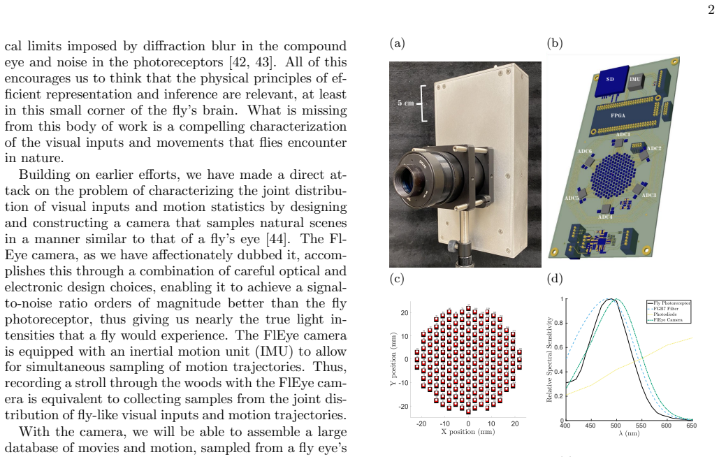
The central object is the FlEye camera itself: 187 silicon PIN photodiodes in a hexagonal lattice with the blowfly's $1.57^\circ$ inter-receptor spacing, masked to circular apertures and placed behind a holographic diffuser and a two-lens system that reproduces the compound eye's Gaussian point-spread function of width about $0.51^\circ$, plus a cyan filter matching the photoreceptor spectral peak near 490 nm. Its effective photon-counting rate exceeds $10^8$ s$^{-1}$, orders of magnitude above the fly's saturation near $10^6$ s$^{-1}$, so the recorded intensities are close to ground truth and fly-like noise can be added later. An inertial measurement unit is synchronized to the photodiodes at the millisecond level, so each frame is paired with pitch, roll, and yaw velocities. The analytic machinery is the conditional-mean estimator $\hat v_\phi = E[v_\phi | \partial_t \ln I, \partial_\phi \ln I, \partial_\theta \ln I]$, evaluated by Monte Carlo binning of the measured joint distribution; slicing this estimator at fixed $\partial_\theta \ln I$ is what exposes both the gradient-to-correlator crossover and the cross-axis noise effect. In that crossover, the gradient estimator, which forms velocity as the ratio of temporal to spatial derivatives, is the high-signal-to-noise limit, while the correlator, which forms velocity from their product, is the low-signal-to-noise limit.
What would settle it
Compute the same conditional-mean estimators from image-and-motion data recorded on a freely flying insect or on a platform driven with fly-like accelerations; if the gradient-to-correlator crossover or the pitch-gradient noise effect changes qualitatively, the naturalistic-sample assumption is refuted. Separately, inspect the connectome of yaw-sensitive lobula-plate neurons: if their inputs do not include photoreceptors separated along the pitch axis, the paper's central neural prediction is refuted.
Extended reading notes
Core claim
The central discovery is that natural movie-and-motion data, collected with a fly-matched camera, support the optimal-estimation picture of fly motion vision and expose a new cross-axis interaction. When yaw velocity is estimated from the local temporal and azimuthal derivatives of log intensity, the conditional-mean estimator $\hat v_\phi = E[v_\phi | \partial_t \ln I, \partial_\phi \ln I]$ has contours that are correlator-like hyperbolae at small derivatives and gradient-like straight lines at large derivatives, with the crossover at derivative magnitudes that occur during an ordinary walk. Conditioning also on the polar derivative $\partial_\theta \ln I$ shows that large $|\partial_\theta \ln I|$, combined with pitch motion, expands the ill-defined central region and makes the yaw-velocity contours noisier, which the authors read as orthogonal gradients acting as noise for yaw estimation. They draw the concrete consequence that yaw-sensitive motion neurons should receive inputs from photoreceptors separated along the pitch axis.
Load-bearing premise
The load-bearing premise is that a 45-minute walk through the woods by a person samples the joint distribution of visual inputs and motions that flies encounter in nature; the paper itself notes (Section IV B) that human walking does not reach the enthusiasm of fly flight, so if fly motion statistics differ substantially, the measured estimator structure, including the pitch-gradient noise effect, may not transfer to the fly.
Editorial extensions
If this is right
- The gradient-to-correlator crossover in optimal local motion estimators is visible in natural data and occurs at derivative values that are common on a real walk, so the predicted systematic errors of motion estimation matter for real vision, not only for toy stimuli.
- Adding simulated photoreceptor noise to the camera's near-noiseless records expands the correlator-like region, qualitatively matching experiments on motion-sensitive neurons; estimation errors are thus consistent with optimal inference in noise rather than a biological flaw.
- Yaw-velocity estimates are degraded by large pitch-direction gradients combined with pitch motion, so nominally orthogonal visual signals are not irrelevant to a given velocity estimate.
- Yaw-sensitive lobula-plate neurons should receive input from photoreceptors separated along the pitch axis, a prediction that can be checked directly against the recently mapped connectome.
- The instrument enables a calibrated database of natural movies paired with ground-truth motion, providing a resource for quantitative tests of adaptation, wide-field motion integration, and coding efficiency in the fly visual system.
Reading between the lines
- The authors do not test whether the cross-axis interaction is reciprocal, but the same estimator construction could check whether pitch-velocity estimates are analogously degraded by large azimuthal gradients, which would strengthen the claim that orthogonal derivatives act as noise.
- Because the training data come from human walking, which the paper itself flags as gentler than fly flight, a natural extension is to record from a camera carried by a free-flying insect or a fast robot; the prediction is that the sizes of the correlator region and the pitch-noise effect shift with motion statistics while the qualitative structure remains.
- The same Monte Carlo conditional-mean approach could be applied to nonlocal features such as pairs or triplets of spatial derivatives, asking how much information local estimators leave on the table compared with wide-field integration.
- Adding calibrated photon shot noise to the stored movies would turn the database into a tunable signal-to-noise dial, allowing a systematic map of the gradient-to-correlator transition and its pitch-axis modulation across light levels.
Editorial analysis
A structured set of objections, weighed in public.
Referee Report
Summary. The paper reports the design, construction, and calibration of the FlEye camera, a portable fly-eye-like imaging system with 187 photodiodes, fly-matched spectral sensitivity and point-spread functions, and a synchronized IMU for motion capture. After characterizing the instrument (PSFs, noise power spectra, transfer functions, effective Poisson rate, and IMU-optical alignment), the authors use a 45-minute walk through a nature preserve to construct optimal local estimators of yaw velocity from temporal and spatial derivatives of log intensity. The two-dimensional estimator reproduces the previously reported gradient-to-correlator crossover, and a three-dimensional extension conditioning also on the polar derivative is used to argue that large polar gradients act as noise for yaw estimation, leading to a prediction about yaw-sensitive connectivity in the fly visual system.
Significance. If the instrument claims stand, this is a valuable contribution: the camera characterization is unusually complete, including measured PSF covariance matrices and skewness, noise power spectra, contrast transfer functions, an effective Poisson rate exceeding 10^8 Hz, and a quantitative IMU-optical alignment check with 0.54 deg/s mean difference. The paper also provides reproducible code and data-processing tools, and it makes a concrete, falsifiable biological prediction. The two-dimensional estimator results are a clear and useful illustration of the instrument's potential. However, the new three-dimensional claim in Section IV C and the resulting Section V prediction currently rest on a binned conditional mean without uncertainty quantification, so the statistical strength of the central new result is not yet established.
major comments (3)
- [IV C, Eq. (13), Fig. 8] The new biological claim rests on the three-dimensional conditional mean in Eq. (13), but Fig. 8 is presented without error bars, confidence intervals, or per-bin sample counts. The text states that conditional means are computed using N=100 equal-sized bins along each axis; if this same binning is used for the three-dimensional estimator, the ~1.35e6 samples available after 500 Hz downsampling give on average about one sample per bin. Because the derivative distributions have nearly exponential tails (Fig. 6b), the high-|∂θ ln I| slices that display the reported 'cone' and 'fuzziness' must contain very few samples. The authors should show, via bootstrap or jackknife confidence intervals, adaptive or coarser binning, or a regularized estimator, that the cone and the loss of definition survive sampling noise; otherwise the qualitative reading of Fig. 8 is not distinguishable from Monte Carlo fluctuations. If a different binning was used for the three-dimensional case, that binning should be stated explicitly.
- [IV C, text after Fig. 8] The statement that 'large gradients in the polar or pitch direction, in combination with pitch movement, act as noise for estimating yaw velocity' is not directly supported by Eq. (13), which conditions on ∂θ ln I but not on any IMU measure of pitch velocity. The estimator in Eq. (13) cannot by itself separate the effect of large polar gradients from the effect of pitch motion, even if the two are correlated in natural data. To support the 'in combination with pitch movement' claim, the authors should include pitch velocity in the conditioning set, or analyze the interaction between ∂θ ln I and measured pitch velocity explicitly. The current analysis only establishes, at best, a dependence of the conditional mean on ∂θ ln I, not the proposed mechanism.
- [IV B / V] The paper acknowledges in Section IV B that 'human walking does not reach the enthusiasm of fly flight,' yet the Section V prediction about yaw-sensitive connectivity is stated without qualification. If fly flight has substantially different joint statistics—for example, higher angular velocities, saccadic head and body movements, or different correlations between pitch and yaw—the orthogonal-gradient interaction observed in the human-walk data may not transfer to the fly. The authors should either temper the connectivity prediction or provide evidence that the estimator structure, especially the ∂θ ln I dependence, is robust across motion statistics, for instance by reweighting the data to better match fly-like movement distributions or by recording under additional natural conditions.
minor comments (5)
- [Introduction] There is a typo in 'large monpoloar cells (LMCs)'; it should read 'large monopolar cells.'
- [Section III B / Eq. (5)] In the text preceding Eq. (5), 'Possion rate' should be 'Poisson rate.'
- [Section II B] The sentence 'the photodiodes were masked to a 1 mm circular active area to remove any affects their square profile had on the PSF' should use 'effects' rather than 'affects.'
- [Appendix C] The heading 'Performance measurements' is misspelled as 'meausurements,' and later in the same appendix 'esitmate' should be 'estimate.'
- [Fig. 4 caption] The caption says 'saturare at λeff ∼ 10^6 Hz'; this should be 'saturate.'
Circularity Check
No significant circularity: the estimator is an empirical conditional mean computed from the recorded data, and the neural-connectivity prediction is an extrapolation beyond the fitted surface.
full rationale
The paper's derivation chain is self-contained. The optimal local motion estimator is defined directly as the conditional mean E[v_phi | derivatives] (Eqs. 11 and 13) and computed by Monte Carlo averaging over the recorded FlEye data; therefore the appearance of gradient-like and correlator-like regions in Fig. 7 is an empirical description of the joint statistics, not a quantity fitted elsewhere and then renamed as a prediction. The new three-dimensional result in Fig. 8 is likewise a direct conditional average, and the Section V statement that yaw-sensitive neurons should receive inputs from pitch-separated photoreceptors is an extrapolation beyond the fitted surface, not a restatement of the regression input. Self-citations [44], [56], and [62] are present, but [44] is used only for comparison with an earlier data set, [56] is a theoretical result motivating the shape of the estimator, and [62] is a peripheral neural hint; removing any of them would not collapse the central claim. The statistical concern about sparse high-|d_theta ln I| slices in Fig. 8 is a robustness and sampling issue for the empirical estimate, not a circularity of the derivation. No step in the paper reduces by construction to its own input.
Assumptions & free parameters
free parameters (3)
- Per-photodiode one-knot quadratic spline coefficients =
theta0-theta4 and knot k1 per photodiode
- Estimator bin count N =
100 bins per derivative axis
- Preprocessing parameters =
2-frame moving average; downsampling to 500 Hz
assumptions (5)
- domain assumption Rigid motion model I(phi,t) = I0(phi - vt)
- standard math Conditional mean minimizes mean-square error
- domain assumption Local spatiotemporal derivatives are sufficient statistics for local velocity estimation
- domain assumption A single 45-minute human walk represents the fly's natural environment
- domain assumption Noise is photon shot noise, Ns(omega) = |T(omega)|^2 / lambda_eff
Cite this review
Pith. "Pith review of The FlEye camera: Sampling the joint distribution of natural scenes and motion." pith.science (2026). https://pith.science/paper/2FWW6AHJ
@misc{pith2026241221081,
  author       = {Pith},
  title        = {Pith review of: The FlEye camera: Sampling the joint distribution of natural scenes and motion},
  year         = {2026},
  howpublished = {\url{https://pith.science/paper/2FWW6AHJ}},
  note         = {Machine review of arXiv:2412.21081}
}
read the original abstract
To make efficient use of limited physical resources, the brain must match its coding and computational strategies to the statistical structure of input signals. An attractive testing ground for these principles is the problem of motion estimation in the fly visual system: we understand the optics of the compound eye, have a quantitative description of input signals and noise from the retina, and can record from output neurons that encode estimates of different velocity components. Furthermore, recent work provides a nearly complete wiring diagram of the intervening circuitry. What is missing is a characterization of the visual signals and motions that flies encounter in a natural context. We attack this directly with the development of a specialized camera that matches the high temporal resolution, optical properties, and spectral sensitivity of the fly's eye; inertial motion sensors provide ground truth about rotations and translations through the world. We describe the design, construction, and performance characteristics of this FlEye camera. To illustrate the opportunities created by this instrument we use data on movies and motion to construct optimal local motion estimators that can be compared with the responses of the fly's motion sensitive neurons.
Figures


Figures from the paper (10 more)


Reference graph
Works this paper leans on
-
[1]
Optical Measurements The photodiode PSF was measured by recording the camera’s responses to a 48 × 48 high intensity LED dis- play with a 500 Hz rate and 12-bit pulse width modula- tion (PWM). Individual display LEDs had a square pro- file with an edge length of 5 mm, giving the full display a height and width of 24 .2 cm. The photodiode PSF and effective...
-
[2]
Signals and noise One of the major design goals of the camera was for it to have a SNR significantly higher than the fly early vi- sual system. In particular, we wanted the camera’s SNR to exceed that of the fly large monopolar cell (LMC), a secondary visual neuron that combines the responses of six photoreceptors. We quantify the camera’s SNR by looking ...
-
[3]
First, a simple rotation test of the FlEye camera on a high precision turntable
Measurements of motion The gyro-optical properties of the camera were mea- sured in two experiments. First, a simple rotation test of the FlEye camera on a high precision turntable. The FlEye camera was centered on the table along one of its main rotational axes. The table was then rotated through a half rotation. The IMU’s response was integrated along t...
-
[4]
H. von Helmholtz, Treatise on Physiological Optics (Op- tical Society of America, Washington DC, 1925) Trans- lated from the 3rd German Edition (1910), by J. P. C. Southall
work page 1910
-
[5]
C. E. Shannon, The Bell System Technical Journal 27, 379 (1948)
1948
-
[6]
N. Wiener, Extrapolation, Interpolation, and Smoothing of Stationary Time Series (John Wiley and Sons, New York, 1949)
work page 1949
-
[7]
J. L. Lawson and G. E. Uhlenbeck, Threshold Signals (McGraw-Hill, New York, 1950) Massachusetts Institute of Technology Radiation Laboratory Series, Volume 24
work page 1950
-
[8]
P. Grassberger and J.-P. Nadal, eds., From Statistical Physics to Statistical Inference and Back (Kluwer, Dor- drecht, 1994)
work page 1994
Show all 68 references
-
[9]
H. B. Barlow, in National Physical Laboratory Sympo- sium on the Mechanization of Thought Processes, Volume 2 (HM Stationery Office, London, 1959) pp. 537–574
1959
-
[10]
Bialek, Biophysics: Searching for Principles (Prince- ton Univerity Press, Princeton NJ, 2012)
W. Bialek, Biophysics: Searching for Principles (Prince- ton Univerity Press, Princeton NJ, 2012)
2012
-
[11]
Bialek, in Les Houches Summer School Lecture Notes: Theoretical Biological Physics 2023, edited by A.-F
W. Bialek, in Les Houches Summer School Lecture Notes: Theoretical Biological Physics 2023, edited by A.-F. Bit- bol, T. Mora, I. Nemenman, and A. M. Walczak (SciPost Physics Lecture Notes, 2024)
2023
-
[12]
S. B. Laughlin, Zeitschrift f¨ ur Naturforschung 36c, 910 (1981)
1981
-
[13]
J. H. van Hateren, Nature 360, 68 (1992)
1992
-
[14]
Rieke, D
F. Rieke, D. Warland, R. de Ruyter van Steveninck, and W. Bialek, Spikes: Exploring the Neural Code (MIT Press, Cambridge MA, 1997)
1997
-
[15]
Brenner, W
N. Brenner, W. Bialek, and R. de Ruyter van Steveninck, Neuron 26, 695 (2000)
2000
-
[16]
D. A. Clark and J. E. Fitzgerald, Annual Review of Vi- sion Science 10, 23 (2024)
2024
-
[17]
Zbikowski, IEEE Instrumentation and Measurement Magazine 7, 19 (2004)
R. Zbikowski, IEEE Instrumentation and Measurement Magazine 7, 19 (2004)
2004
-
[18]
Dickson, A
W. Dickson, A. Straw, C. Poelma, and M. Dickinson, in 44th AIAA Aerospace Sciences Meeting and Exhibit (2006) p. 34
2006
-
[19]
G. K. Taylor and H. G. Krapp, Advances in Insect Phys- iology 34, 231 (2007)
2007
-
[20]
J. C. Tuthill and R. I. Wilson, Current Biology26, R1022 (2016)
2016
-
[21]
Lehmann and J
F.-O. Lehmann and J. Bartussek, Journal of Compara- tive Physiology A 203, 1 (2017)
2017
-
[22]
B. H. Dickerson, Proceedings of the Royal Society B 287, 20201774 (2020)
2020
-
[23]
W. B. Dickson, A. D. Straw, and M. H. Dickinson, AIAA Journal 46, 2150 (2008)
2008
-
[24]
S. C. Whitehead, S. Leone, T. Lindsay, M. R. Meiselman, N. J. Cowan, M. H. Dickinson, N. Yapici, D. L. Stern, T. Shirangi, and I. Cohen, Science Advances 8, eabo7461 (2022)
2022
-
[25]
de Ruyter van Steveninck and S
R. de Ruyter van Steveninck and S. B. Laughlin, Inter- national Journal of Neural Systems 7, 437 (1996)
1996
-
[26]
D. Cao, A. J. Zele, and J. Pokorny, Vision Research 47, 1060 (2007)
2007
-
[27]
D. G. Stavenga, Journal of Comparative Physiology A 189, 189 (2003)
2003
-
[28]
H. B. Barlow, The Journal of Experimental Biology 29, 667 (1952)
1952
-
[29]
D. G. Stavenga, Journal of Comparative Physiology A 189, 1 (2003)
2003
-
[30]
D. G. Stavenga, Journal of Comparative Physiology A 190, 115 (2004)
2004
-
[31]
P. G. Lillywhite, Journal of Comparative Physiology A 122, 189 (1977)
1977
-
[32]
R. R. de Ruyter van Steveninck and S. B. Laughlin, Na- ture 379, 642 (1996)
1996
-
[33]
Pierantoni, Cell and Tissue Research 171, 101 (1976)
R. Pierantoni, Cell and Tissue Research 171, 101 (1976)
1976
-
[34]
Hausen, in Photoreception and Vision in Inverte- brates, edited by M
K. Hausen, in Photoreception and Vision in Inverte- brates, edited by M. A. Ali (Springer, 1984) pp. 523–559
1984
-
[35]
H. G. Krapp, Navigation 55, 147 (2008)
2008
-
[36]
S. J. Huston and H. G. Krapp, PLoS Biology 6, e173 (2008)
2008
-
[37]
T. W. Ullrich, R. Kern, and M. Egelhaaf, Biology Open 4, 13 (2014)
2014
-
[38]
R. D. Williams, T. L. Massey, and M. M. Maharbiz, in 2018 40th Annual International Conference of the IEEE Engineering in Medicine and Biology Society (EMBC) (IEEE, 2018) pp. 1685–1688
2018
-
[39]
H. Wei, H. Y. Kyung, P. J. Kim, and C. Desplan, Journal of Comparative Physiology A 206, 139 (2020)
2020
-
[40]
S Dorkenwald, A
A. S Dorkenwald, A. Matsliah, A. R. Sterling, P. Schlegel, S.-C. Yu, C. E. McKellar, A. Lin, M. Costa, K. Eich- ler, Y. Yin, W. Silversmith, C. Schneider-Mizell, C. S. Jordan, D. Brittain, A. Halageri, K. Kuehner, O. Oge- dengbe, R. Morey, J. Gager, K. Kruk, E. Perlman, R. Yan...
2024
-
[41]
de Ruyter van Steveninck and W
R. de Ruyter van Steveninck and W. Bialek, in Mod- els of Neural Networks IV: Early Vision and Attention (Springer–Verlag, 2002) pp. 313–365
2002
-
[42]
Nemenman, G
I. Nemenman, G. D. Lewen, W. Bialek, and R. R. de Ruyter van Steveninck, PLoS Computational Biology 4, e1000025 (2008)
2008
-
[43]
M. S. Drews, A. Leonhardt, N. Pirogova, F. G. Richter, A. Schuetzenberger, L. Braun, E. Serbe, and A. Borst, Current Biology 30, 209 (2020)
2020
-
[44]
A. L. Fairhall, G. D. Lewen, W. Bialek, and R. de Ruyter van Steveninck, Nature 412, 787 (2001)
2001
-
[45]
Bialek, F
W. Bialek, F. Rieke, R. R. de Ruyter van Steven inck, and D. Warland, Science 252, 1854 (1991)
1991
-
[46]
de Ruyter van Steveninck and W
R. de Ruyter van Steveninck and W. Bialek, Philosophi- cal Transactions of the Royal Society of London348, 321 (1995)
1995
-
[47]
S. R. Sinha, W. Bialek, and R. R. de Ruyter van Steveninck, Physical Review Letters 126, 018101 (2021)
2021
-
[48]
Merrifield and L
S. Merrifield and L. Wilkinson, SimpleSDHC, https:// github.com/ibm2030/SimpleSDHC (2000)
2000
-
[49]
Beersma, D
D. Beersma, D. Stavenga, and J. Kuiper, Journal of com- parative physiology 119, 207 (1977)
1977
-
[50]
J. G. J. Smakman, J. H. van Hateren, and D. G. Stavenga, Journal of Comparative Physiology A155, 239 (1984)
1984
-
[51]
C. J. Edelson, MCRayTracing, https://github.com/ edelsonc/MCRayTracing (2024)
2024
-
[52]
Limb and J
J. Limb and J. Murphy, Computer Graphics and Image 16 Processing 4, 311 (1975)
1975
-
[53]
Reichardt, in Symposium on Principles of Sensory Communication 1959 (MIT Press, Cambridge MA, 1961) pp
W. Reichardt, in Symposium on Principles of Sensory Communication 1959 (MIT Press, Cambridge MA, 1961) pp. 303–317
1959
-
[54]
E. H. Adelson and J. R. Bergen, Journal of the Optical Society of America A 2, 284 (1985)
1985
-
[55]
Reichardt and T
W. Reichardt and T. Poggio, Quarterly Reviews of Bio- physics 9, 311 (1976)
1976
-
[56]
Egelhaaf, A
M. Egelhaaf, A. Borst, and W. Reichardt, Journal of the Optical Society of America A 6, 1070 (1989)
1989
-
[57]
de Ruyter van Steveninck, W
R. de Ruyter van Steveninck, W. Bialek, M. Potters, and R. Carlson, in Proceedings of IEEE International Con- ference on Systems, Man and Cybernetics , Vol. 1 (IEEE,
-
[58]
J. P. Van Santen and G. Sperling, Journal of the Optical Society of America A 1, 451 (1984)
1984
-
[59]
Potters and W
M. Potters and W. Bialek, Journal de Physique I 4, 1755 (1994)
1994
-
[60]
Weiss, E
Y. Weiss, E. P. Simoncelli, and E. H. Adelson, Nature Neuroscience 5, 598 (2002)
2002
-
[61]
A. A. Stocker and E. P. Simoncelli, Nature Neuroscience 9, 578 (2006)
2006
-
[62]
D. C. Knill and W. Richards, Perception as Bayesian Inference (Cambridge University Press, 1996)
1996
-
[63]
C. J. Edelson, FlEye Reader, https://github.com/ edelsonc/FlEye_Reader (2024)
2024
-
[64]
R. R. de Ruyter van Steveninck, W. Bialek, M. Potters, R. H. Carlson, and G. D. Lewen, in Natural and artifi- cial parallel computation, Proc. of the 5th NEC Research Symposium, edited by D. L. Waltz (SIAM, 1996) pp. 21– 41
1996
-
[65]
S. Roy, S. R. Sinha, and R. R de Ruyter van Steveninck, Journal of Neuroscience 35, 6481 (2015)
2015
-
[66]
Wertheimer, Zeitschrift f¨ ur Psychologie61, 161–265 (1912)
M. Wertheimer, Zeitschrift f¨ ur Psychologie61, 161–265 (1912)
1912
-
[67]
Hassenstein and W
B. Hassenstein and W. Reichardt, Zeitschrift f¨ ur Natur- forschung B 11B, 513 (1956)
1956
-
[68]
J. C. Lagarias, J. A. Reeds, M. H. Wright, and P. E. Wright, SIAM Journal on Optimization 9, 112 (1998)
1998
Reviewed August 10, 2026 · model on record in the stance chip above.
Discussion (0). Continue with ORCID to comment.