REVIEW 3 major objections 5 minor 45 references
Closed-form random-matrix bounds tie the noise-induced error of reconstructive spectrometers to spectral correlation length, mean transmittance, and channel counts, and show super-resolution below the correlation limit is a signal-to-noise
Reviewed by Pith at T0; open to challenge. T0 means a machine referee read the full paper against a public rubric. the ladder, T0–T4 →
T0 review · deepseek-v4-flash
2026-08-03 14:22 UTC pith:PFWVV24B
load-bearing objection A genuinely useful closed-form bound for reconstructive spectrometers, with a solid over-determined branch and a softer underdetermined branch that is still credible thanks to independent full-wave validation. the 3 major comments →
Resolution and Robustness Bounds for Reconstructive Spectrometers
The pith
A machine-rendered reading of the paper's core claim, the machinery that carries it, and where it could break.
Core claim
The paper's central claim is that the noise-induced mean squared error (MSE) of spectral reconstruction is set by the Cramér–Rao lower bound σ_ε² Tr[(A^T A)^+], and that for generic chaotic scatterers with Lorentzian speckle correlations this trace obeys a closed-form ensemble average. In the over-determined regime (M ≥ N), E[Tr(G+)] = (M N/|M−N|) J(a)/T0², with a = Γcorr/Δω and J(a) a monotone function that grows exponentially for a ≳ 1; in the under-determined regime (M < N), a modified function J̃(a) replaces J(a) through an effective correlation length a_eff = √2 (M/N) a. From this, the effective spectral resolution Δωmin follows as approximately πΓcorr / ln R_SNR in the over-determined
What carries the argument
The load-bearing identity is the closed-form expression for the inverse trace of the Gram matrix, E[Tr(G+)] = (M N/|M−N|) J(a)/T0² (with a modified J̃ for M<N). It is assembled from three pieces: (i) the Fisher information / Cramér–Rao lower bound, which identifies σ_ε² Tr(G+) as the variance floor; (ii) the statistical model of the transmission matrix, where A^T A ≈ C, with C a near-Toeplitz matrix of Lorentzian form C_ij = T0² a²/((i−j)²+a²) reflecting Rayleigh speckle and a Lorentzian spectral correlation function; and (iii) Szegő's theorem for Toeplitz matrices, which turns the trace of C^+ into an integral over the reciprocal of the generating function, yielding the function J(a). The f
Load-bearing premise
The entire closed-form structure — the J(a) function, the √2 M/N factor, and the super-resolution formula — assumes the scatterer obeys conventional Rayleigh speckle statistics with a Lorentzian spectral correlation function; when a device deviates from this (as inverse-designed structures do), the predicted numerical bounds no longer apply.
What would settle it
Measure the minimum resolvable frequency spacing Δωmin of a fixed reconstructive spectrometer as the detector noise σ_ε is varied over several orders of magnitude; the theory predicts Δωmin ∝ 1/ln(const/σ_ε²). A power-law or saturating dependence on σ_ε would falsify the super-resolution formula, provided Γcorr, T0, M, and N are held fixed and the speckle correlations are confirmed to be Lorentzian.
If this is right
- Designers can estimate the noise-limited MSE of a candidate spectrometer directly from Γcorr, T0, M, N, and σ_ε, without simulating the reconstruction algorithm.
- Super-resolution below the spectral correlation length is not a design contradiction; it is achievable provided the effective SNR R_SNR exceeds the threshold set by the resolution target.
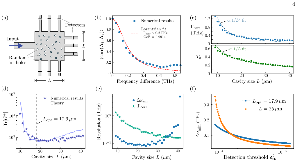
- There is an optimal device size for a given scattering platform, arising from the opposite scalings of T0 and Γcorr with length; the paper predicts it from the closed-form bound.
- The bound is algorithm-independent for small noise: both pseudoinverse and neural-network reconstruction exhibit the same noise-induced MSE in that regime, so the formula is a robust design target.
- In the under-determined regime, the resolution formula carries an extra √2 M/N factor, meaning the ratio of measurement to frequency channels directly enters the achievable super-resolution.
Where Pith is reading between the lines
- The derivation of the under-determined broadening factor η≈√2 is calibrated against the same random-matrix ensemble used for validation; an independent derivation from the Fejér convolution integral would strengthen the prediction for intermediate M/N, where the fit might drift.
- Because the bound relies only on Lorentzian speckle statistics, the same closed form should apply to other speckle-based spectrometer platforms (multimode fibers, photonic chips, quantum-dot films) as long as their intensity correlations remain Lorentzian — a testable prediction across device classes.
- The inverse-design result shows that intentionally non-Lorentzian correlations can beat the random-scatterer bound, suggesting that engineering the dwell-time distribution of the cavity is a more powerful route to super-resolution than simply shortening Γcorr.
Editorial analysis
A structured set of objections, weighed in public.
Referee Report
Summary. The paper develops a theory for the noise-induced reconstruction error of speckle-based reconstructive spectrometers. Starting from a Gaussian noise model and the Cramér–Rao lower bound, it argues that the variance floor is σ_ϵ² Tr[(AᵀA)⁺]. Assuming chaotic-scattering (Rayleigh/speckle) statistics and Lorentzian spectral correlations, it models the correlation matrix C as a near-Toeplitz matrix with entries T₀² a²/((i−j)²+a²), where a = Γ_corr/Δω. Using Szegő's theorem, it derives a closed-form expression for E[Tr(G⁺)] in the over-determined (M≥N) case, Eq. (12), and proposes a modified scaling function J̃(a) for the under-determined case, Eq. (14)–(15). These formulas lead to super-resolution conditions, Eqs. (13) and (16). The theory is validated against a Mahaux–Weidenmüller random-matrix ensemble and full-wave FDTD simulations of a disordered cavity, with additional tests on neural-network reconstruction and an inverse-design study.
Significance. If the central relations (12) and (15) hold, the paper provides a physically grounded design tool: reconstruction error is expressed through measurable quantities (correlation length, mean transmittance, channel counts), and the analysis identifies trade-offs between these parameters, including an optimal device size. The over-determined branch is built on standard Toeplitz/Szegő theory and is well supported by numerical tests. The paper also makes a useful conceptual point that Γ_corr alone does not set the resolution limit; effective SNR matters. The machine-checkable, reproducible numerical validation and the explicit admission of the Lorentzian assumption are strengths.
major comments (3)
- [Supplemental S4, Eqs. (S18)–(S21); main Eqs. (14)–(16)] The under-determined scaling function J̃(a) rests on an ansatz whose shape parameter is fitted rather than derived. Equation (S18) sets a_eff = ηβa, and the text states that comparison with the RMT ensemble in the a≫1 limit gives η≈√2. This same RMT ensemble family is later used as the validation set in Fig. 2(c). The agreement in Fig. 2(c) therefore does not independently confirm the value of η. Because Eq. (16) and the full-wave optimal-size prediction in Fig. 3(d)–(e) rely on this under-determined branch, the quantitative super-resolution predictions inherit the uncertainty in η. I request either an independent derivation of η from the Fejér-kernel convolution or a validation on a structurally different ensemble/device family.
- [Main text, Eqs. (13) and (16); Supplemental S6] The step from the trace formula to the resolution formula is under-derived. The text says 'we straightforwardly obtain' Eq. (13), but the derivation is not shown: the relation between the detection threshold δ_th², the trace bound, and the minimum resolvable spacing Δω_min is nontrivial, especially because the asymptotic J(a) contains prefactors (4a² in the denominator) that are dropped in Eq. (13). If Eq. (13) is meant as a heuristic order-of-magnitude estimate, this should be stated explicitly; if it is meant as a quantitative bound, a derivation must be provided. This is load-bearing because the super-resolution claim is one of the central messages.
- [Main text, Eqs. (5)–(8)] There is a normalization ambiguity in the definition of C. Equation (5) defines C = aᵀa, where each column a_i is an M-vector, so C_ij is an inner product scaling with M. Equation (8) then sets C_ij = T₀² a²/((i−j)²+a²), which is normalized to a unit peak and does not display the factor M. The supplemental text says the factor M is 'absorbed' into the convention, but this is not stated in the main text. Since Eq. (12) is derived from the trace of C⁺, the missing M factor can create dimensional inconsistencies. Please clarify the convention in Eq. (7) or (8).
minor comments (5)
- [Main text, Eq. (6)] The statement that the rank-1 term Nµᵀµ modifies the inverse 'negligibly' for large N should be justified or replaced by a more precise condition; as written, it is plausible but not demonstrated.
- [Main text, Eq. (14)] The argument of the tan⁻¹ in J̃(a) retains tanh(πa/2), while the sinh term uses the rescaled argument. A sentence explaining why the broadening affects only the sinh term would help the reader.
- [Fig. 1(d)] The legend refers to a 'green line', but the figure appears to use a solid line that is not clearly green. Please ensure color/line descriptions match the rendered figure.
- [Supplemental S3] The phrase 'absorbing M into the definition of C_ij as per standard RMT convention' is confusing because C was already defined in Eq. (5). Define the rescaled matrix explicitly, e.g., C̃_ij = C_ij/M.
- [Main text, Eq. (12)] The sentence 'The M/(M−N) factor arises from the Marchenko–Pastur distribution' is cryptic; include the standard result or a reference to the relevant limiting form.
Circularity Check
Under-determined branch calibrates η≈√2 on the same RMT ensemble later used as validation; full-wave tests provide partial independent support.
specific steps
-
fitted input called prediction
[Supplemental Material S4 (Eqs. S18–S21), used in main-text Eqs. (14)–(16) and Fig. 2(c)]
"By comparing to the RMT ensemble in the limit of strong correlations (a≫1), we find that the broadening factor converges to η≈√2—i.e., the Bartlett windowing broadens the effective spectral correlation width by a factor of √2 relative to a hard rectangular truncation. Thus, we set a_eff=√2 (M/N) a."
The under-determined scaling function is introduced as an ansatz (a_eff=ηβa), and the shape parameter η is fixed numerically by comparison to the RMT ensemble. No derivation of η≈√2 from the stated Fejér/Bartlett convolution is provided. The same Mahaux–Weidenmüller RMT model is then used as the validation ensemble in Fig. 2(c) and S2, so the agreement of Eq. (15)/(16) with those RMT points is not an independent check of the fitted shape parameter. This makes the under-determined branch a calibrated interpolation rather than a parameter-free first-principles result. The over-determined formula is not affected, and the full-wave FDTD simulations give partial external support, but the central 'super-resolution' Eq. (16) inherits the calibrated η.
full rationale
The central Fisher-information bound and the over-determined J(a) formula are independently grounded: the Cramér–Rao bound is standard estimation theory, Eqs. (10)–(11) follow from Toeplitz/Szegő theory, and the Lorentzian correlation is an explicit modeling assumption. The only load-bearing circular step is in S4: η≈√2 is calibrated on the same RMT ensemble family used for validation, so the under-determined branch (Eqs. 14–16) is not fully derived from the stated convolution argument. The paper does, however, test the theory against full-wave FDTD simulations (Fig. 3), which are independent of the RMT calibration, and it explicitly flags the Lorentzian-speckle assumption as non-universal in the conclusion and S7 inverse-design study. Self-citations such as Ref. [41] appear in the outlook/inverse-design discussion and are not load-bearing for the main derivation. Overall, the circularity is real but localized; the main over-determined predictions and the external full-wave comparison carry independent content.
Axiom & Free-Parameter Ledger
free parameters (1)
- η (underdetermined broadening factor) =
√2 ≈ 1.414 (inferred from RMT ensemble fit)
axioms (6)
- domain assumption Measurement noise is independent additive Gaussian with identical variance σ_epsilon^2 (Eq. 1).
- domain assumption Intensity statistics are Rayleigh (negative exponential) with standard deviation equal to mean transmittance T0 (S3, Eq. S6).
- domain assumption Spectral correlations decay as a Lorentzian in frequency separation (Eq. 8 and S3, Eq. S13).
- domain assumption A^T A approximately follows Wishart/Marchenko–Pastur statistics so that E[Tr(G+)] gains the M/|M−N| prefactor (footnote [37]).
- domain assumption The trace of the pseudoinverse is approximated by its expectation over the ensemble, ignoring fluctuations around the mean Toeplitz form (Eq. 10, Szegő theorem).
- ad hoc to paper Ansatz a_eff = η β a with η=√2 for the underdetermined case (S4, Eq. S18).
read the original abstract
Reconstructive spectrometers are a promising emerging class of devices that combine complex light scattering with inference to enable compact, high-resolution spectrometry. Thus far, the physical determinants of these devices' performance remain under-explored. We show that under a broad range of conditions, the noise-induced error for spectral reconstruction is governed by the Fisher information. We then use random matrix theory to derive a closed-form relation linking the variance bound to a set of key physical parameters: the spectral correlation length, the mean transmittance, and the number of frequency and measurement channels. The analysis reveals certain fundamental trade-offs between these physical parameters, and establishes the conditions for a spectrometer to achieve ``super-resolution'' below the limit set by the spectral correlation length. Our theory is confirmed using numerical validations with a random matrix model as well as full-wave simulations. These results establish a physically-grounded framework for designing and analyzing performant and noise-robust reconstructive spectrometers.
Figures


Reference graph
Works this paper leans on
-
[1]
S. P. Davis, M. C. Abrams, and J. W. Brault,Fourier transform spectrometry(Academic press, 2001)
2001
-
[2]
Redding, S
B. Redding, S. F. Liew, R. Sarma, and H. Cao, Com- pact spectrometer based on a disordered photonic chip, Nature Photonics7, 746 (2013)
2013
-
[3]
Momeni, E
B. Momeni, E. S. Hosseini, M. Askari, M. Soltani, and A. Adibi, Integrated photonic crystal spectrometers for sensing applications, Optics communications282, 3168 (2009)
2009
-
[4]
Z. Xia, A. A. Eftekhar, M. Soltani, B. Momeni, Q. Li, M. Chamanzar, S. Yegnanarayanan, and A. Adibi, High resolution on-chip spectroscopy based on miniaturized microdonut resonators, Optics express19, 12356 (2011)
2011
-
[5]
T. Yang, C. Xu, H.-p. Ho, Y.-y. Zhu, X.-h. Hong, Q.-j. Wang, Y.-c. Chen, X.-a. Li, X.-h. Zhou, M.-d. Yi,et al., Miniature spectrometer based on diffraction in a disper- sive hole array, Optics letters40, 3217 (2015)
2015
-
[6]
Z. Yang, T. Albrow-Owen, W. Cai, and T. Hasan, Miniaturization of optical spectrometers, Science371, eabe0722 (2021). 6
2021
-
[7]
Zhang, J
L. Zhang, J. Chen, C. Ma, W. Li, Z. Qi, and N. Xue, Re- search progress on on-chip fourier transform spectrome- ter, Laser & Photonics Reviews15, 2100016 (2021)
2021
-
[8]
Redding and H
B. Redding and H. Cao, Using a multimode fiber as a high-resolution, low-loss spectrometer, inFiber Optic Sensors and Applications XI, Vol. 9098 (SPIE, 2014) pp. 89–93
2014
-
[9]
S. F. Liew, B. Redding, M. A. Choma, H. D. Tagare, and H. Cao, Broadband multimode fiber spectrometer, Optics letters41, 2029 (2016)
2029
-
[10]
Bao and M
J. Bao and M. G. Bawendi, A colloidal quantum dot spec- trometer, Nature523, 67 (2015)
2015
-
[11]
Faraji-Dana, E
M. Faraji-Dana, E. Arbabi, A. Arbabi, S. M. Kamali, H. Kwon, and A. Faraon, Compact folded metasurface spectrometer, Nature communications9, 4196 (2018)
2018
-
[12]
Z. Yang, T. Albrow-Owen, H. Cui, J. Alexander-Webber, F. Gu, X. Wang, T.-C. Wu, M. Zhuge, C. Williams, P. Wang,et al., Single-nanowire spectrometers, Science 365, 1017 (2019)
2019
-
[13]
D.-G. Lee, G. Song, C. Lee, C. Lee, and M. Jang, Re- constructive spectrometer using double-layer disordered metasurfaces, Science Advances11, eadv2376 (2025)
2025
-
[14]
D. A. Miller, Waves, modes, communications, and optics: a tutorial, Advances in Optics and Photonics11, 679 (2019)
2019
-
[15]
H. H. Yoon, H. A. Fernandez, F. Nigmatulin, W. Cai, Z. Yang, H. Cui, F. Ahmed, X. Cui, M. G. Uddin, E. D. Minot,et al., Miniaturized spectrometers with a tunable van der waals junction, Science378, 296 (2022)
2022
-
[16]
G. Cai, Y. Li, Y. Zhang, X. Jiang, Y. Chen, G. Qu, X. Zhang, S. Xiao, J. Han, S. Yu,et al., Compact angle- resolved metasurface spectrometer, Nature Materials23, 71 (2024)
2024
-
[17]
Varytis, D.-N
P. Varytis, D.-N. Huynh, W. Hartmann, W. Pernice, and K. Busch, Design study of random spectrometers for ap- plications at optical frequencies, Optics Letters43, 3180 (2018)
2018
-
[18]
B. R. Frieden,Physics from Fisher information: a unifi- cation(Cambridge University Press, 1998)
1998
-
[19]
Y. V. Fyodorov, Random matrix theory of resonances: An overview, in2016 URSI International Symposium on Electromagnetic Theory (EMTS)(IEEE, 2016) pp. 666– 669
2016
-
[20]
Lehmann, D
N. Lehmann, D. Saher, V. Sokolov, and H.-J. Sommers, Chaotic scattering: the supersymmetry method for large number of channels, Nuclear Physics A582, 223 (1995)
1995
-
[21]
Y. V. Fyodorov and H.-J. Sommers, Statistics of reso- nance poles, phase shifts and time delays in quantum chaotic scattering: Random matrix approach for systems with broken time-reversal invariance, Journal of Mathe- matical Physics38, 1918 (1997)
1918
-
[22]
S. M. Popoff, G. Lerosey, R. Carminati, M. Fink, A. C. Boccara, and S. Gigan, Measuring the transmission ma- trix in optics: An approach to the study and control of light propagation in disordered media, Physical review letters104, 100601 (2010)
2010
-
[23]
Goetschy and A
A. Goetschy and A. Stone, Filtering random matrices: the effect of incomplete channel control in multiple scat- tering, Physical review letters111, 063901 (2013)
2013
-
[24]
Cao and J
H. Cao and J. Wiersig, Dielectric microcavities: Model systems for wave chaos and non-hermitian physics, Re- views of Modern Physics87, 61 (2015)
2015
-
[25]
Akkermans and G
E. Akkermans and G. Montambaux,Mesoscopic physics of electrons and photons(Cambridge university press, 2007)
2007
-
[26]
See supplementary material (2025), see online Supple- mental Materials
2025
-
[27]
S. M. Kay,Fundamentals of statistical signal processing: estimation theory(Prentice-Hall, Inc., 1993)
1993
-
[28]
R. J. Ober, Q. Zou, and Z. Lin, Calculation of the fisher information matrix for multidimensional data sets, IEEE transactions on signal processing51, 2679 (2003)
2003
-
[29]
L. S. Rothman, R. R. Gamache, A. Goldman, L. R. Brown, R. A. Toth, H. M. Pickett, R. L. Poynter, J.- M. Flaud, C. Camy-Peyret, A. Barbe,et al., The hitran database: 1986 edition, Applied optics26, 4058 (1987)
1986
-
[30]
Sherman and W
J. Sherman and W. J. Morrison, Adjustment of an inverse matrix corresponding to a change in one element of a given matrix, The Annals of Mathematical Statistics21, 124 (1950)
1950
-
[31]
J. W. Goodman,Speckle phenomena in optics: the- ory and applications(Roberts and Company Publishers, 2007)
2007
-
[32]
Ericson, Fluctuations of nuclear cross sections in the” continuum” region, Physical Review Letters5, 430 (1960)
T. Ericson, Fluctuations of nuclear cross sections in the” continuum” region, Physical Review Letters5, 430 (1960)
1960
-
[33]
Weidenm¨ uller and G
H. Weidenm¨ uller and G. Mitchell, Random matrices and chaos in nuclear physics: Nuclear structure, Reviews of Modern Physics81, 539 (2009)
2009
-
[34]
R. M. Grayet al., Toeplitz and circulant matrices: A review, Foundations and Trends in Communications and Information Theory2, 155 (2006)
2006
-
[35]
B¨ ottcher and B
A. B¨ ottcher and B. Silbermann,Analysis of Toeplitz op- erators(Springer, 2006)
2006
-
[36]
Hirschman Jr, The strong szeg¨ o limit theorem for toeplitz determinants, American Journal of Mathemat- ics , 577 (1966)
I. Hirschman Jr, The strong szeg¨ o limit theorem for toeplitz determinants, American Journal of Mathemat- ics , 577 (1966)
1966
-
[37]
Strictly speaking, the scattering matrices in the Mahaux– Weidenm¨ uller model are not Wishart, but they approx- imately satisfy Wishart statistics in the chaotic regime with strong mode overlap
-
[38]
A. M. Tulino, S. Verd´ u,et al., Random matrix theory and wireless communications, Foundations and Trends in Communications and Information Theory1, 1 (2004)
2004
-
[39]
Molesky, Z
S. Molesky, Z. Lin, A. Y. Piggott, W. Jin, J. Vuckovi´ c, and A. W. Rodriguez, Inverse design in nanophotonics, Nature Photonics12, 659 (2019)
2019
-
[40]
Kroker, S
S. Kroker, S. Lanteri, O. Miller, J. Niegemann, and L. Ra- munno, Inverse design in photonics: introduction, J. Opt. Soc. Am. B41, IDP1 (2024)
2024
-
[41]
J. Yu, H. Lo, W. Chen, C. Zhu, Y. Wu, F. Wang, C. Wang, C. Yan, C. Dang, B. Wen,et al., Wavelength- scale noise-resistant on-chip spectrometer, arXiv preprint arXiv:2509.22286 (2025)
arXiv 2025
-
[42]
Lakshminarayan, S
A. Lakshminarayan, S. Tomsovic, O. Bohigas, and S. N. Majumdar, Extreme statistics of complex random and quantum chaotic states, Phys. Rev. Lett.100, 044103 (2008)
2008
-
[43]
Performance Bounds for Reconstructive Spectrometers
A. Chabanov, M. Stoytchev, and A. Genack, Statisti- cal signatures of photon localization, Nature404, 850 (2000). 7 Supplemental Materials for “Performance Bounds for Reconstructive Spectrometers” S1. DA T ASET PREP ARA TION AND RECONSTRUCTION ALGORITHMS Dataset preparation—In our numerical simulations, the ground truth spectrum samples are drawn from a d...
2000
-
[44]
The estimator is ˆx=A +y, whereA + =A T (AAT )−1
The Moore-Penrose pseudoinverse. The estimator is ˆx=A +y, whereA + =A T (AAT )−1. This linear reconstruc- tion scheme serves as the baseline for the theoretical analysis based on Fisher information and the Cram´ er–Rao bound
-
[45]
resolution
A fully-connected neural network (NN), implemented using the PyTorch framework. The NN comprises three hidden layers of 500 neurons each. Each layer is followed by a ReLU activation, dropout regularization, and batch normalization to enhance training stability and mitigate overfitting. Training is done using the Adam optimizer with a learning rate of 1×10...
discussion (0)
Sign in with ORCID, Apple, or X to comment. Anyone can read and Pith papers without signing in.