Recognition: 2 theorem links
· Lean TheoremConditional flow matching for physics-constrained inverse problems with finite training data
Pith reviewed 2026-05-15 10:53 UTC · model grok-4.3
The pith
A neural network learns the velocity field of a conditional probability flow ODE that transports source samples directly to the measurement-conditioned posterior in physics inverse problems.
A machine-rendered reading of the paper's core claim, the machinery that carries it, and where it could break.
Core claim
Conditional flow matching trains a neural network to learn the velocity field of a probability flow ordinary differential equation that transports samples from a chosen source distribution directly to the posterior distribution conditioned on observed measurements, without requiring explicit evaluation of the prior and likelihood densities.
What carries the argument
The conditional velocity field of the probability flow ODE, parameterized by a neural network and trained via the flow-matching objective on joint samples.
If this is right
- The approach accommodates nonlinear and non-differentiable physics forward models.
- Multimodal posteriors are recovered without explicit density evaluations.
- Early stopping on held-out test loss prevents variance collapse and selective memorization.
- Both Gaussian and data-informed source distributions can be used as starting points for transport.
- Computational cost remains low compared with repeated forward-model evaluations inside traditional sampling methods.
Where Pith is reading between the lines
- The same transport mechanism could be applied to other conditional sampling tasks where only paired data are observed.
- Selective memorization implies that performance will degrade on test measurements far from the training distribution unless the source is chosen to cover the relevant range.
- The method offers a route to amortize posterior sampling once the network is trained, enabling rapid inference on new measurements.
Load-bearing premise
Samples from the joint distribution of inferred variables and measurements are available.
What would settle it
Run the trained conditional flow model on a synthetic inverse problem whose true posterior is known analytically or by exhaustive sampling and check whether the generated samples reproduce the correct multimodal structure and marginal variances.
Figures


read the original abstract
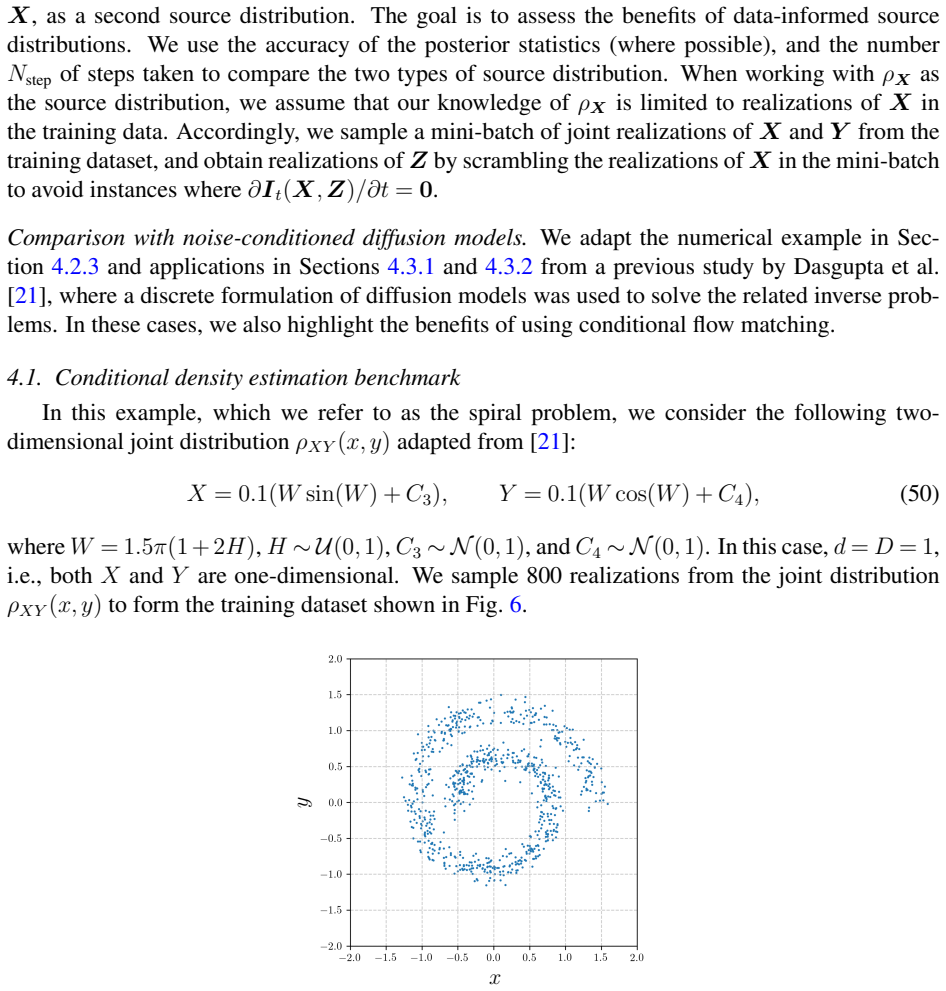
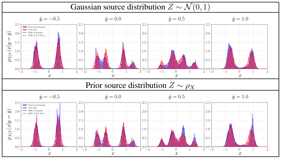
This study presents a conditional flow matching framework for solving physics-constrained Bayesian inverse problems. In this setting, samples from the joint distribution of inferred variables and measurements are assumed available, while explicit evaluation of the prior and likelihood densities is not required. We derive a simple and self-contained formulation of both the unconditional and conditional flow matching algorithms, tailored specifically to inverse problems. In the conditional setting, a neural network is trained to learn the velocity field of a probability flow ordinary differential equation that transports samples from a chosen source distribution directly to the posterior distribution conditioned on observed measurements. This black-box formulation accommodates nonlinear, high-dimensional, and potentially non-differentiable forward models without restrictive assumptions on the noise model. We further analyze the behavior of the learned velocity field in the regime of finite training data. Under mild architectural assumptions, we show that overtraining can induce degenerate behavior in the generated conditional distributions, including variance collapse and a phenomenon termed selective memorization, wherein generated samples concentrate around training data points associated with similar observations. A simplified theoretical analysis explains this behavior, and numerical experiments confirm it in practice. We demonstrate that standard early-stopping criteria based on monitoring test loss effectively mitigate such degeneracy. The proposed method is evaluated on several physics-based inverse problems. We investigate the impact of different choices of source distributions, including Gaussian and data-informed priors. Across these examples, conditional flow matching accurately captures complex, multimodal posterior distributions while maintaining computational efficiency.
Editorial analysis
A structured set of objections, weighed in public.
Referee Report
Summary. The paper presents a conditional flow matching framework for physics-constrained Bayesian inverse problems. Assuming joint samples of inferred variables and measurements are available (but not explicit prior/likelihood densities), it derives unconditional and conditional flow-matching objectives, trains a neural network to learn the velocity field of a probability-flow ODE that transports source samples directly to the conditional posterior p(x|y*), analyzes finite-data degeneracy (selective memorization and variance collapse) under mild architectural assumptions, shows that early-stopping on held-out test loss mitigates these effects, and validates the approach on several physics-based inverse problems with different source distributions.
Significance. If the finite-data analysis and mitigation hold, the method supplies a practical, black-box sampler for multimodal posteriors in high-dimensional nonlinear inverse problems without density evaluations or differentiability assumptions on the forward model. This could be useful for settings with limited joint training pairs and complex physics simulators.
major comments (1)
- [Finite-data analysis] Finite-data analysis (abstract and associated section): the assertion that early-stopping on unconditional held-out test loss reliably prevents selective memorization for out-of-sample y* is load-bearing for the central finite-data claim. The test loss does not directly penalize mismatch between the generated conditional law and the true posterior; a concrete diagnostic (e.g., posterior predictive checks or mode-recovery metrics on held-out y*) is needed to confirm the stopped network recovers modes rather than merely interpolating training pairs.
minor comments (2)
- Abstract and methods: no equations for the conditional velocity field, no network architecture details, and no description of how the velocity is optimized are provided; these must be added for reproducibility.
- Experiments: report error bars or multiple runs when claiming accurate capture of multimodal posteriors; clarify quantitative metrics used to assess posterior fidelity.
Simulated Author's Rebuttal
We thank the referee for their constructive and insightful review. The major comment on the finite-data analysis raises a valid point about the indirect nature of the test loss, and we address it directly below while outlining the revisions we will make.
read point-by-point responses
-
Referee: [Finite-data analysis] Finite-data analysis (abstract and associated section): the assertion that early-stopping on unconditional held-out test loss reliably prevents selective memorization for out-of-sample y* is load-bearing for the central finite-data claim. The test loss does not directly penalize mismatch between the generated conditional law and the true posterior; a concrete diagnostic (e.g., posterior predictive checks or mode-recovery metrics on held-out y*) is needed to confirm the stopped network recovers modes rather than merely interpolating training pairs.
Authors: We agree with the referee that the unconditional held-out test loss serves as an indirect proxy and does not explicitly measure fidelity of the generated conditional distribution to the true posterior for unseen y*. Our theoretical analysis (under the stated mild architectural assumptions) demonstrates that overtraining induces selective memorization and variance collapse by driving the velocity field to map source samples toward training pairs with similar observations. The early-stopping rule is motivated by the fact that the minimum of the unconditional test loss occurs before this degeneracy sets in, and our numerical experiments across multiple physics inverse problems show that the resulting models recover multimodal structure for out-of-sample y*. Nevertheless, to make this claim more robust, we will add in the revised manuscript explicit diagnostics on held-out y* values: posterior predictive checks (comparing simulated measurements from generated samples against observed y*) and quantitative mode-recovery metrics (e.g., number of recovered modes via clustering and Wasserstein-2 distance to reference posterior samples obtained by long-run MCMC). These additions will directly confirm that the stopped network captures posterior modes rather than merely interpolating training data. revision: yes
Circularity Check
Derivation self-contained from joint samples; no reduction to fitted inputs or self-citation chains
full rationale
The paper derives the unconditional and conditional flow matching objectives directly from available joint samples of (x, y) pairs, without explicit prior/likelihood densities. The velocity field is regressed to the conditional vector field implied by the probability flow ODE, and the finite-data degeneracy analysis (variance collapse, selective memorization) follows from the regression objective under mild architectural assumptions. Early-stopping is justified by monitoring the same test loss that defines the training objective, with numerical confirmation on physics examples. No load-bearing step reduces by construction to a fitted parameter renamed as prediction, nor relies on self-citation for uniqueness or ansatz. The formulation is presented as black-box and self-contained, keeping the central claim independent of its inputs.
Axiom & Free-Parameter Ledger
axioms (1)
- domain assumption Joint samples of inferred variables and measurements are available
Lean theorems connected to this paper
-
IndisputableMonolith/Cost/FunctionalEquation.leanwashburn_uniqueness_aczel unclear?
unclearRelation between the paper passage and the cited Recognition theorem.
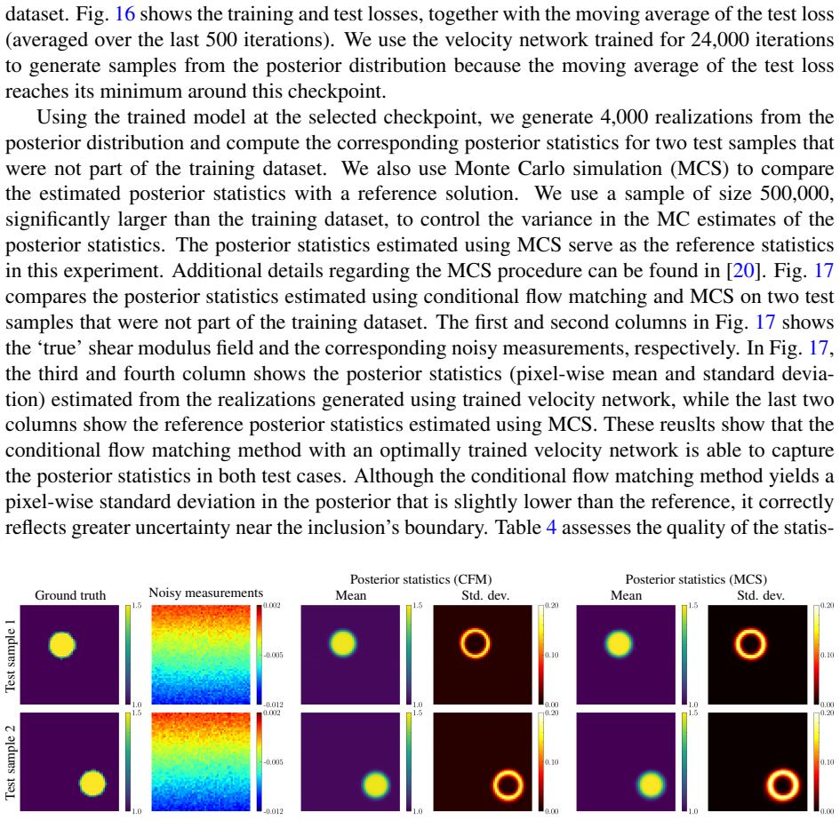
the loss function for the velocity field is given by Eq. (20)... minimizer of ˆL(bt) is equal to the minimizer of L(bt)
-
IndisputableMonolith/Foundation/BranchSelection.leanbranch_selection unclear?
unclearRelation between the paper passage and the cited Recognition theorem.
overtraining can induce degenerate behavior... selective memorization... variance collapse
What do these tags mean?
- matches
- The paper's claim is directly supported by a theorem in the formal canon.
- supports
- The theorem supports part of the paper's argument, but the paper may add assumptions or extra steps.
- extends
- The paper goes beyond the formal theorem; the theorem is a base layer rather than the whole result.
- uses
- The paper appears to rely on the theorem as machinery.
- contradicts
- The paper's claim conflicts with a theorem or certificate in the canon.
- unclear
- Pith found a possible connection, but the passage is too broad, indirect, or ambiguous to say the theorem truly supports the claim.
Reference graph
Works this paper leans on
-
[1]
A. M. Stuart, Inverse problems: a Bayesian perspective, Acta numerica 19 (2010) 451–559
work page 2010
-
[2]
D. Calvetti, E. Somersalo, Inverse problems: From regularization to Bayesian inference, Wiley Interdisciplinary Reviews: Computational Statistics 10 (2018) e1427
work page 2018
-
[3]
L. Tierney, J. B. Kadane, Accurate approximations for posterior moments and marginal densities, Journal of the american statistical association 81 (1986) 82–86
work page 1986
-
[4]
S. Brooks, Markov chain Monte Carlo method and its application, Journal of the royal statistical society: series D (the Statistician) 47 (1998) 69–100
work page 1998
-
[5]
R. M. Neal, et al., MCMC using Hamiltonian dynamics, Handbook of markov chain monte carlo 2 (2011) 2
work page 2011
-
[6]
A. G. Dimakis, A. Bora, D. Van Veen, A. Jalal, S. Vishwanath, E. Price, Deep generative models and inverse problems, Mathematical Aspects of Deep Learning 400 (2022)
work page 2022
-
[7]
S. Lunz, O. ¨Oktem, C.-B. Sch¨onlieb, Adversarial regularizers in inverse problems, Advances in neural informa- tion processing systems 31 (2018)
work page 2018
- [8]
-
[9]
M. Duff, N. D. Campbell, M. J. Ehrhardt, Regularising inverse problems with generative machine learning models, Journal of Mathematical Imaging and Vision 66 (2024) 37–56
work page 2024
-
[10]
D. V . Patel, D. Ray, A. A. Oberai, Solution of physics-based Bayesian inverse problems with deep generative priors, Computer Methods in Applied Mechanics and Engineering 400 (2022) 115428
work page 2022
-
[11]
D. Ray, J. Murgoitio-Esandi, A. Dasgupta, A. A. Oberai, Solution of physics-based inverse problems using conditional generative adversarial networks with full gradient penalty, Computer Methods in Applied Mechanics and Engineering 417 (2023) 116338
work page 2023
- [12]
-
[13]
P. Hagemann, J. Hertrich, G. Steidl, Stochastic normalizing flows for inverse problems: A Markov chains viewpoint, SIAM/ASA Journal on Uncertainty Quantification 10 (2022) 1162–1190
work page 2022
-
[14]
A. Dasgupta, D. V . Patel, D. Ray, E. A. Johnson, A. A. Oberai, A dimension-reduced variational approach for solving physics-based inverse problems using generative adversarial network priors and normalizing flows, Computer Methods in Applied Mechanics and Engineering 420 (2024) 116682
work page 2024
- [15]
- [16]
-
[17]
H. Wang, X. Zhang, T. Li, Y . Wan, T. Chen, J. Sun, DMPlug: A plug-in method for solving inverse problems with diffusion models, Advances in Neural Information Processing Systems 37 (2024) 117881–117916
work page 2024
-
[18]
Conditional image generation with score-based diffusion models.arXiv preprint arXiv:2111.13606,
G. Batzolis, J. Stanczuk, C.-B. Sch ¨onlieb, C. Etmann, Conditional image generation with score-based diffusion models, arXiv preprint arXiv:2111.13606 (2021)
-
[19]
C. Jacobsen, Y . Zhuang, K. Duraisamy, COCOGEN: Physically consistent and conditioned score-based gener- ative models for forward and inverse problems, SIAM Journal on Scientific Computing 47 (2025) C399–C425
work page 2025
-
[20]
A. Dasgupta, H. Ramaswamy, J. Murgoitio-Esandi, K. Y . Foo, R. Li, Q. Zhou, B. F. Kennedy, A. A. Oberai, Conditional score-based diffusion models for solving inverse elasticity problems, Computer Methods in Applied Mechanics and Engineering 433 (2025) 117425
work page 2025
-
[21]
A. Dasgupta, A. Marciano da Cunha, A. Fardisi, M. Aminy, B. Binder, B. Shaddy, A. A. Oberai, Unifying and extending diffusion models through PDEs for solving inverse problems, Computer Methods in Applied Mechanics and Engineering 448 (2026) 118431
work page 2026
- [22]
- [23]
-
[24]
J. Tauberschmidt, S. Fellenz, S. J. V ollmer, A. B. Duncan, Physics-constrained fine-tuning of flow-matching models for generation and inverse problems, arXiv preprint arXiv:2508.09156 (2025)
-
[25]
U. Utkarsh, P. Cai, A. Edelman, R. Gomez-Bombarelli, C. V . Rackauckas, Physics-constrained flow matching: Sampling generative models with hard constraints, arXiv preprint arXiv:2506.04171 (2025)
-
[26]
I. J. Goodfellow, J. Pouget-Abadie, M. Mirza, B. Xu, D. Warde-Farley, S. Ozair, A. Courville, Y . Bengio, Generative adversarial nets, Advances in neural information processing systems 27 (2014)
work page 2014
-
[27]
M. Arjovsky, S. Chintala, L. Bottou, Wasserstein generative adversarial networks, in: International conference on machine learning, PMLR, 2017, pp. 214–223
work page 2017
-
[28]
I. Kobyzev, S. J. Prince, M. A. Brubaker, Normalizing flows: An introduction and review of current methods, IEEE transactions on pattern analysis and machine intelligence 43 (2020) 3964–3979
work page 2020
-
[29]
L. Dinh, D. Krueger, Y . Bengio, NICE: Non-linear independent components estimation, arXiv preprint arXiv:1410.8516 (2014)
work page internal anchor Pith review Pith/arXiv arXiv 2014
-
[30]
L. Dinh, J. Sohl-Dickstein, S. Bengio, Density estimation using Real NVP, arXiv preprint arXiv:1605.08803 (2016)
work page internal anchor Pith review Pith/arXiv arXiv 2016
-
[31]
R. T. Chen, Y . Rubanova, J. Bettencourt, D. K. Duvenaud, Neural ordinary differential equations, Advances in neural information processing systems 31 (2018)
work page 2018
-
[32]
J. Ho, A. Jain, P. Abbeel, Denoising diffusion probabilistic models, Advances in neural information processing systems 33 (2020) 6840–6851
work page 2020
-
[33]
J. Sohl-Dickstein, E. Weiss, N. Maheswaranathan, S. Ganguli, Deep unsupervised learning using nonequilibrium thermodynamics, in: International conference on machine learning, pmlr, 2015, pp. 2256–2265
work page 2015
-
[34]
Y . Song, J. Sohl-Dickstein, D. P. Kingma, A. Kumar, S. Ermon, B. Poole, Score-based generative modeling through stochastic differential equations, arXiv preprint arXiv:2011.13456 (2020)
work page internal anchor Pith review Pith/arXiv arXiv 2011
-
[35]
Flow Matching for Generative Modeling
Y . Lipman, R. T. Chen, H. Ben-Hamu, M. Nickel, M. Le, Flow matching for generative modeling, arXiv preprint arXiv:2210.02747 (2022)
work page internal anchor Pith review Pith/arXiv arXiv 2022
-
[36]
X. Liu, C. Gong, Q. Liu, Flow straight and fast: Learning to generate and transfer data with rectified flow, arXiv preprint arXiv:2209.03003 (2022)
work page internal anchor Pith review Pith/arXiv arXiv 2022
-
[37]
M. S. Albergo, E. Vanden-Eijnden, Building normalizing flows with stochastic interpolants, arXiv preprint arXiv:2209.15571 (2022)
work page internal anchor Pith review Pith/arXiv arXiv 2022
- [38]
-
[39]
J. Wildberger, M. Dax, S. Buchholz, S. Green, J. H. Macke, B. Sch ¨olkopf, Flow matching for scalable simulation-based inference, Advances in Neural Information Processing Systems 36 (2023) 16837–16864. 48
work page 2023
-
[40]
L. Lu, P. Jin, G. Pang, Z. Zhang, G. E. Karniadakis, Learning nonlinear operators via DeepONet based on the universal approximation theorem of operators, Nature machine intelligence 3 (2021) 218–229
work page 2021
-
[41]
D. Ray, O. Pinti, A. A. Oberai, Deep Learning and Computational Physics, Springer, 2024
work page 2024
-
[42]
R. Baptista, A. Dasgupta, N. B. Kovachki, A. Oberai, A. M. Stuart, Memorization and regularization in genera- tive diffusion models, arXiv preprint arXiv:2501.15785 (2025)
-
[43]
A. Paszke, S. Gross, F. Massa, A. Lerer, J. Bradbury, G. Chanan, T. Killeen, Z. Lin, N. Gimelshein, L. Antiga, A. Desmaison, A. Kopf, E. Yang, Z. DeVito, M. Raison, A. Tejani, S. Chilamkurthy, B. Steiner, L. Fang, J. Bai, S. Chintala, PyTorch: An imperative style, high-performance deep learning library, in: Advances in Neural Information Processing System...
work page 2019
-
[44]
D. P. Kingma, J. Ba, Adam: A method for stochastic optimization, International Conference on Learning Representations (ICLR) (2015)
work page 2015
-
[45]
P. Virtanen, R. Gommers, T. E. Oliphant, M. Haberland, T. Reddy, D. Cournapeau, E. Burovski, P. Peterson, W. Weckesser, J. Bright, S. J. van der Walt, M. Brett, J. Wilson, K. J. Millman, N. Mayorov, A. R. J. Nelson, E. Jones, R. Kern, E. Larson, C. J. Carey,˙I. Polat, Y . Feng, E. W. Moore, J. VanderPlas, D. Laxalde, J. Perktold, R. Cimrman, I. Henriksen,...
work page 2020
-
[46]
M. Cuturi, Sinkhorn distances: Lightspeed computation of optimal transport, Advances in Neural Information Processing Systems 27 (2013) 2292 – 2300
work page 2013
-
[47]
G. Evensen, The ensemble kalman filter: Theoretical formulation and practical implementation, Ocean dynam- ics 53 (2003) 343–367
work page 2003
- [48]
-
[49]
E. N. Lorenz, Deterministic nonperiodic flow, Journal of Atmospheric Sciences 20 (1963) 130 – 141
work page 1963
-
[50]
K.-Y . Lam, S. Liu, Y . Lou, Selected topics on reaction-diffusion-advection models from spatial ecology, Mathe- matics in Applied Sciences and Engineering 1 (2020) 91–206. URL:https://ojs.lib.uwo.ca/index. php/mase/article/view/10644. doi:10.5206/mase/10644
-
[51]
A. Logg, K.-A. Mardal, G. N. Wells, et al., Automated Solution of Differential Equations by the Finite Element Method, Springer, 2012. doi:10.1007/978-3-642-23099-8
-
[52]
P. E. Barbone, A. A. Oberai, A review of the mathematical and computational foundations of biomechanical imaging, Computational Modeling in Biomechanics (2009) 375–408
work page 2009
-
[53]
T. Z. Pavan, E. L. Madsen, G. R. Frank, J. Jiang, A. A. Carneiro, T. J. Hall, A nonlinear elasticity phantom containing spherical inclusions, Physics in medicine & biology 57 (2012) 4787
work page 2012
-
[54]
B. F. Kennedy, K. M. Kennedy, D. D. Sampson, A review of Optical Coherence Elastography: Fundamentals, Techniques and Prospects, IEEE Journal of Selected Topics in Quantum Electronics 20 (2014) 272–288
work page 2014
-
[55]
B. F. Kennedy, R. A. McLaughlin, K. M. Kennedy, L. Chin, A. Curatolo, A. Tien, B. Latham, C. M. Saunders, D. D. Sampson, Optical coherence micro-elastography: mechanical-contrast imaging of tissue microstructure, Biomedical optics express 5 (2014) 2113–2124
work page 2014
-
[56]
K. Y . Foo, B. Shaddy, J. Murgoitio-Esandi, M. S. Hepburn, J. Li, A. Mowla, D. Vahala, S. E. Amos, Y . S. Choi, A. A. Oberai, K. B. F, Tumor spheroid elasticity estimation using mechano-microscopy combined with a conditional generative adversarial network, Computer Methods and Programs in Biomedicine (2024) 108362
work page 2024
-
[57]
E. R. Ferreira, A. A. Oberai, P. E. Barbone, Uniqueness of the elastography inverse problem for incompressible nonlinear planar hyperelasticity, Inverse problems 28 (2012) 065008. 49
work page 2012
discussion (0)
Sign in with ORCID, Apple, or X to comment. Anyone can read and Pith papers without signing in.