The Illusion of Stochasticity in LLMs
Pith reviewed 2026-05-10 18:48 UTC · model grok-4.3
The pith
LLMs cannot map their internal probability estimates to accurate stochastic outputs when sampling from distributions.
A machine-rendered reading of the paper's core claim, the machinery that carries it, and where it could break.
Core claim
The paper establishes that LLMs suffer from a fundamental mismatch: while they can use provided random seeds to produce outputs matching target distributions, their direct sampling from specific distributions does not reflect their internal probability estimates, exposing a core limitation in emulating stochastic processes required for agentic behavior.
What carries the argument
The mismatch between LLMs' internal probability estimates over tokens and the empirical distributions of their generated stochastic outputs during direct sampling tasks.
If this is right
- Agentic LLM systems will need external sampling modules to achieve reliable stochastic behavior.
- Even frontier models exhibit the sampling failure across multiple distributions and prompting methods.
- Tasks requiring sampling from inferred data distributions will show systematic deviations from intended behavior.
- LLMs cannot replace standard RL agents in environments that depend on independent random sampling.
Where Pith is reading between the lines
- Training regimes that explicitly include stochastic sampling objectives might reduce the mismatch without changing the base architecture.
- This limitation could extend to related capabilities like uncertainty estimation or simulation-based reasoning in LLMs.
- Hybrid systems combining LLMs with dedicated random number generators may become standard for agent deployments.
Load-bearing premise
The mismatch between internal probability estimates and generated outputs is a fundamental architectural or training limitation rather than a fixable artifact of prompting or insufficient exposure to stochastic tasks.
What would settle it
A test where samples generated by an LLM from a known distribution, without any external random seeds, produce an empirical frequency distribution that closely matches the model's own reported token probabilities for that task.
Figures
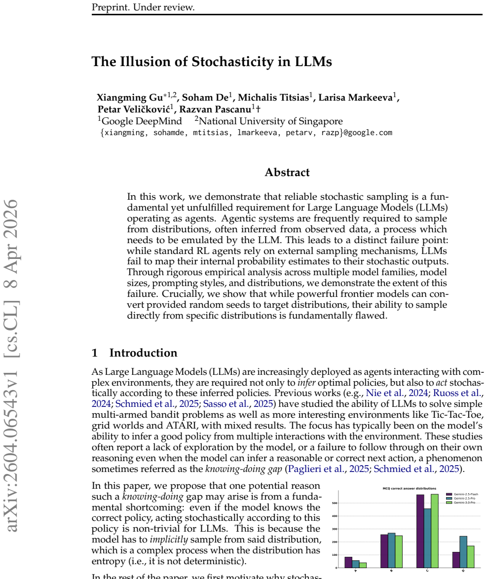


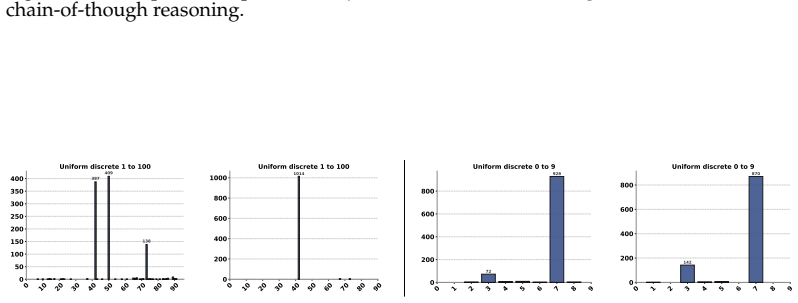


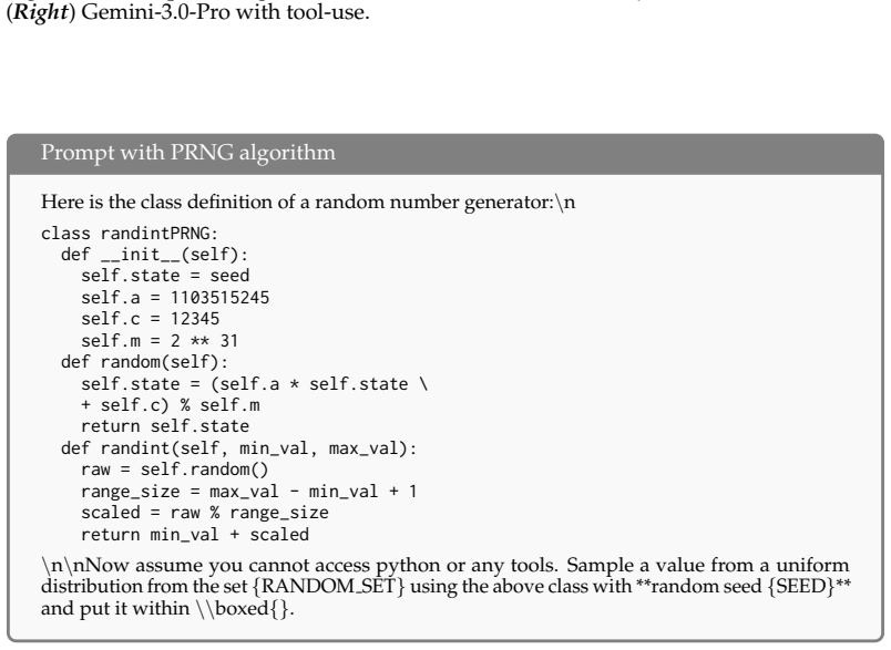


read the original abstract
In this work, we demonstrate that reliable stochastic sampling is a fundamental yet unfulfilled requirement for Large Language Models (LLMs) operating as agents. Agentic systems are frequently required to sample from distributions, often inferred from observed data, a process which needs to be emulated by the LLM. This leads to a distinct failure point: while standard RL agents rely on external sampling mechanisms, LLMs fail to map their internal probability estimates to their stochastic outputs. Through rigorous empirical analysis across multiple model families, model sizes, prompting styles, and distributions, we demonstrate the extent of this failure. Crucially, we show that while powerful frontier models can convert provided random seeds to target distributions, their ability to sample directly from specific distributions is fundamentally flawed.
Editorial analysis
A structured set of objections, weighed in public.
Referee Report
Summary. The paper claims that LLMs cannot reliably perform direct stochastic sampling from target probability distributions (despite internal probability estimates), while they succeed at converting externally provided random seeds into samples from those distributions. This distinction is presented as a fundamental limitation for agentic use of LLMs, supported by empirical tests across model families, sizes, prompting styles, and distributions.
Significance. If substantiated, the result would highlight a practical barrier to using LLMs for tasks requiring unbiased sampling from inferred distributions, reinforcing the need for external randomness sources in agent architectures rather than relying on the model's token-generation process.
major comments (2)
- [Abstract] Abstract: the assertion of 'rigorous empirical analysis across multiple model families, model sizes, prompting styles, and distributions' supplies no sample sizes, specific distributions tested, evaluation metrics for mismatch between internal probabilities and outputs, or statistical controls, making it impossible to assess whether the data support the claim that direct sampling is 'fundamentally flawed'.
- [Abstract] The central distinction between seed-assisted and direct sampling is load-bearing, yet the manuscript does not describe controls that isolate architectural limits from prompting artifacts (e.g., whether chain-of-thought or distribution-specific few-shot examples were systematically varied).
Simulated Author's Rebuttal
We thank the referee for their constructive comments, which highlight opportunities to improve the clarity and transparency of our empirical claims. We address each major comment point by point below, indicating revisions where we agree the manuscript can be strengthened.
read point-by-point responses
-
Referee: [Abstract] Abstract: the assertion of 'rigorous empirical analysis across multiple model families, model sizes, prompting styles, and distributions' supplies no sample sizes, specific distributions tested, evaluation metrics for mismatch between internal probabilities and outputs, or statistical controls, making it impossible to assess whether the data support the claim that direct sampling is 'fundamentally flawed'.
Authors: We agree that the abstract, being concise by nature, does not enumerate these details. The full manuscript (Sections 3 and 4) specifies the experimental scale, the concrete distributions evaluated, the quantitative mismatch metrics (e.g., total variation and KL divergence between target and realized output distributions), and the statistical procedures employed (repeated trials with variance reporting). We have revised the abstract to include a brief summary of sample sizes, distributions, metrics, and controls so that the strength of the evidence can be assessed from the abstract alone. revision: yes
-
Referee: [Abstract] The central distinction between seed-assisted and direct sampling is load-bearing, yet the manuscript does not describe controls that isolate architectural limits from prompting artifacts (e.g., whether chain-of-thought or distribution-specific few-shot examples were systematically varied).
Authors: The manuscript states that results hold across prompting styles and includes those variations in the experimental design. To make the isolation of architectural versus prompting effects fully explicit, we have added a dedicated paragraph in the methods section that systematically enumerates the prompting conditions tested (direct, chain-of-thought, and distribution-specific few-shot) and reports that the performance gap between direct and seed-assisted sampling remains consistent across all variants. This addition clarifies that the observed limitation is not reducible to prompting artifacts. revision: yes
Circularity Check
No significant circularity
full rationale
The paper advances an empirical claim based on experiments across model families, sizes, prompting styles, and distributions: LLMs can map provided random seeds to target distributions but fail at direct sampling from those distributions. No equations, derivations, fitted parameters, or self-referential constructions appear in the abstract or description. The analysis relies on external benchmarks (observed outputs vs. internal probabilities) rather than reducing any result to its own inputs by construction, making the work self-contained.
Axiom & Free-Parameter Ledger
Lean theorems connected to this paper
-
IndisputableMonolith/Foundation/RealityFromDistinction.leanreality_from_one_distinction unclear?
unclearRelation between the paper passage and the cited Recognition theorem.
Crucially, we show that while powerful frontier models can convert provided random seeds to target distributions, their ability to sample directly from specific distributions is fundamentally flawed.
-
IndisputableMonolith/Cost/FunctionalEquation.leanwashburn_uniqueness_aczel unclear?
unclearRelation between the paper passage and the cited Recognition theorem.
LLMs fail to map their internal probability estimates to their stochastic outputs.
What do these tags mean?
- matches
- The paper's claim is directly supported by a theorem in the formal canon.
- supports
- The theorem supports part of the paper's argument, but the paper may add assumptions or extra steps.
- extends
- The paper goes beyond the formal theorem; the theorem is a base layer rather than the whole result.
- uses
- The paper appears to rely on the theorem as machinery.
- contradicts
- The paper's claim conflicts with a theorem or certificate in the canon.
- unclear
- Pith found a possible connection, but the passage is too broad, indirect, or ambiguous to say the theorem truly supports the claim.
Reference graph
Works this paper leans on
-
[1]
A standard fair coin (one Head, one Tail)
-
[2]
A two-headed coin (Heads on both sides)
-
[3]
A coin is selected at random from the bag and flipped
A two-tailed coin (Tails on both sides). A coin is selected at random from the bag and flipped. The coin lands showing **Heads**. What is the probability that the other side of the coin is also Heads? A) 1 3 B) 1 2 C) 2 3 D) 5 6 *** **Correct Answer:** C *** **Explanation:** ... Figure 10: Example responses of (Left) Gemini-2.5-Pro and (Right) Gemini-3.0-...
work page 2025
-
[4]
There’s no bias; the choice is random enough for this operation
It’s perfectly valid given the constraints. There’s no bias; the choice is random enough for this operation. Finally, I’ll format the output within the LaTeX command ‘\\boxed{}‘. Model response:7 Figure 12: Example of thinking trace of Gemini-2.5-Flash when sampling from a uniform discrete distribution between 0 and 9. B.4 Effects of chain-of-thoughts Cur...
-
[5]
Square it: 1234 2 = 1522756. 3. Extract the middle four digits: **2275**. 4. Take this modulo 26: 2275 mod 26=13. 5. Map 13 to the corresponding letter: **m**— Final Answerm Figure 17: Example of response of Qwen3-14B when sampling from a uniform discrete distribution on letters. Qwen3-32B Sample a number from a uniform distribution within the continuous ...
work page 2024
-
[6]
First, we instantiate the class with the given seed
Initialization. First, we instantiate the class with the given seed
-
[7]
Step 1: Get the raw large number by call- ing ‘next raw()‘
Calling ‘randint(0, 9)‘ ... Step 1: Get the raw large number by call- ing ‘next raw()‘ ... ‘(a * state + c) % m‘ ... ‘1103515245 * 1000 = 1103515245000‘ ... ‘1103515245000 + 12345 = 1103515257345‘ ... ‘1103515257345 / 2147483648‘ gives a quotient of ‘513‘ and a remainder ... ‘self.state = 1856145921‘ ... Step 2: Determine the size of the range ... Step 3:...
-
[8]
**Initialize the PRNG with seed 1035**
-
[9]
**Compute the raw number via ‘next raw()‘** ... state= (a·state+c) modm ... First compute: a·state= 1103515245 · 1035 = 1142138278575 ... Then add c: 1142138278575 + 12345 = 1142138290920 ... Now compute modulo m: 1142138290920 mod 2147483648 = 1824473832
-
[10]
Computes: scaled= 1824473832 mod 10 = 2, Returns:result= 0 + 2 = 2
**Generate a number in the range [0, 9]** ... Computes: scaled= 1824473832 mod 10 = 2, Returns:result= 0 + 2 = 2 ... **Final Result** ... 2 Figure 40: Truncated responses when prompting (Left) Gemini-2.5-Pro and (Right) Qwen3- 8B to simulate a PRNG algorithm for uniform discrete distribution between 0 and 9. The thinking traces and some special tokens are...
-
[11]
Initialize the state and constants
-
[12]
Calculate the next state: ... ‘(a * state + c) % m‘ ... Step 2a: ‘a * state‘ ... ‘1103515245 * 1846 = 2037089142270‘ ... Step 2b: ‘a * state + c‘ ... ‘2037089142270 + 12345 = 2037089154615‘ ... Step 2c: ‘(a * state + c) % m‘ ... The remain- der is ‘2037089154615 - 2035814498304 = 1274656311‘
-
[13]
‘1274656311 / 2147483648 ≈ 0.5935603845‘
Normalize the state to get the final number: ... ‘1274656311 / 2147483648 ≈ 0.5935603845‘ ... approximately 0.59356 ... 0.5935603845 . Qwen3-14B ... Sample a number from a uniform dis- tribution within the continuous range [0, 1] ... **random seed 1817** ... [...thinking...] To generate a random number from a uni- form distribution in the continuous range...
-
[14]
‘R‘ = ‘sqrt(3.149)‘ ≈ **1.7746**
**Calculate R:** ... ‘R‘ = ‘sqrt(3.149)‘ ≈ **1.7746** ... 2. **Calculate theta:** ... ‘theta‘≈ **2.5626** (in radians) ... 3. **Cal- culate the final value ‘z0‘: ... ‘z0‘ ≈ **- 1.4832 ... ‘mu + Z * sigma‘, which is ‘0 + z0 * 1‘, the final result is ‘z0‘.−1.4832 Qwen3-32B ... Sample a number from a Gaussian dis- tribution with mean 0 and standard devi- ati...
work page 2023
-
[15]
Convert to float: u2 = 1732512723 2147483648 ≈ 0.807
Resulting state: state2 =1732512723 ... Convert to float: u2 = 1732512723 2147483648 ≈ 0.807 ... Step 3: Apply the Box-Muller Transform ... 1. Compute: R= p −2·ln(u 1) =p −2·ln(0.547)≈ p −2·(−0.603) =√ 1.206≈ 1.098 ... 2. Compute: θ= 2π· u2 = 2π· 0.807 ≈ 5.073 radians ... 3. Com- pute: Z=R·cos(θ)≈ 1.098 ·cos( 5.073) ... 4. Compute cos(5.073)5.073, textrad...
-
[16]
Given ‘u = 0.8921795677048454‘:
and take the floor of the result. Given ‘u = 0.8921795677048454‘:
-
[17]
Multiply by the number of out- comes (10): ‘0.8921795677048454 * 10 = 8.921795677048454‘
-
[18]
Take the floor of the result: ‘floor(8.921795677048454) = 8‘ This method works by dividing the in- terval [0, 1] into 10 equal sub-intervals: [0, 0.1), [0.1, 0.2), ..., [0.9, 1.0). The given number 0.8921795677048454 falls into the interval [0.8, 0.9), which corresponds to the integer 8. The sampled value is 8. 8 Qwen3-30B-A3B Here is a random number samp...
discussion (0)
Sign in with ORCID, Apple, or X to comment. Anyone can read and Pith papers without signing in.