Self-averaging parameter estimation for coarse-grained particle models
Pith reviewed 2026-05-10 03:45 UTC · model grok-4.3
The pith
Coupling a coarse-grained SDE to its own parameter equations produces self-averaging that matches selected microscopic and mesoscopic observables.
A machine-rendered reading of the paper's core claim, the machinery that carries it, and where it could break.
Core claim
The paper claims that the coupled system consisting of the coarse-grained stochastic differential equation with free parameters and the auxiliary dynamic equations for those parameters self-averages, according to Anosov-Kifer's theorem, so that the final parameter values make the averages and correlations of selected observables coincide between the microscopic and mesoscopic descriptions.
What carries the argument
The central mechanism is the self-averaging property of the augmented dynamical system formed by the coarse-grained SDE together with the parameter-evolution equations, which enforces observable matching without external optimization.
If this is right
- The method determines both static parameters appearing in the reversible part of the dynamics, such as those in the free-energy function or potential of mean force, and dynamic parameters such as friction coefficients.
- It identifies state-dependent transport properties, for instance the position-dependent form of the mobility tensor for hydrodynamically interacting particles.
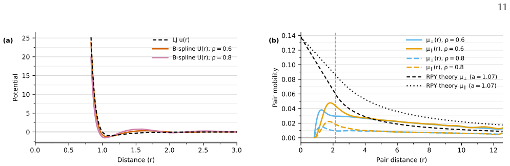
- Application to a bimodal-mass Lennard-Jones fluid infers both the potential of mean force between the heavy particles and its hydrodynamic mobility tensor.
- The procedure is not restricted to constant parameters and extends directly to position-dependent coefficients.
Where Pith is reading between the lines
- If the self-averaging convergence holds for a broader class of observables, the technique could be used to derive coarse-grained models for molecular systems without presupposing functional forms for interactions or transport.
- One could test convergence rates by applying the method to analytically solvable coarse-graining problems and measuring how quickly parameters stabilize.
- The dynamical adjustment of parameters might connect to other adaptive model-reduction approaches by offering an explicit time-evolution route to consistency between scales.
Load-bearing premise
The coupled system of the coarse-grained stochastic differential equation and the parameter-evolution equations self-averages to parameter values that make the chosen microscopic observables coincide with their mesoscopic counterparts.
What would settle it
Running the coupled system for the Brownian particle in a harmonic potential and verifying whether the converged friction and spring-constant parameters reproduce the known microscopic values within numerical error would falsify the claim if they fail to match.
Figures




read the original abstract
We introduce a parameter estimation method that utilizes microscopic data, specifically averages and correlations of selected microscopic observables, to determine the parameters of a stochastic differential equation governing coarse-grained degrees of freedom. The method is not limited to static parameters found in the reversible part of the coarse-grained dynamics, such as those in the free energy function or potential of mean force, but also extends to dynamic parameters, including friction coefficients. The method couples the stochastic differential equation with free parameters to dynamic equations for the parameters. The coupled system self-averages, according to Anosov-Kifer's theorem, in such a way that the final state of the parameters gives coincidence between the microscopic and mesoscopic averages and correlations of selected observables. The method is validated in two examples: a Brownian particle in a harmonic potential, and a set of Brownian particles interacting hydrodynamically with the Rotne-Prager-Yamakawa mobility tensor. This latter case illustrates how the method can be used not only to determine coefficients but also state dependent transport properties - in this case, the position dependent form of the mobility tensor. The parameter estimation for these two models yields excellent results. Subsequently we use the methodology to study a bimodal-mass Lennard-Jones fluid for which we infer both the potential of mean force between the heavy particles and its hydrodynamic mobility tensor.
Editorial analysis
A structured set of objections, weighed in public.
Referee Report
Summary. The paper introduces a parameter estimation method for coarse-grained stochastic differential equations (SDEs) by coupling the SDE (with free parameters) to auxiliary dynamic equations for those parameters. The coupled system is claimed to self-average, per Anosov-Kifer's theorem, such that the parameters converge to values making selected microscopic averages and correlations coincide with their mesoscopic counterparts. The approach is validated on a Brownian particle in a harmonic potential and on hydrodynamically interacting particles using the Rotne-Prager-Yamakawa (RPY) mobility tensor (including inference of its position-dependent form); it is then applied to a bimodal-mass Lennard-Jones fluid to recover both the potential of mean force between heavy particles and the associated hydrodynamic mobility tensor.
Significance. If the self-averaging convergence holds, the method supplies a systematic, non-optimization-based route to infer both static (free-energy/PMF) and dynamic (friction/mobility) parameters from microscopic data. The extension to state-dependent transport coefficients is a clear strength, and the use of a rigorous theorem for justification distinguishes it from purely heuristic matching schemes.
major comments (2)
- [Abstract and validation sections] Abstract and validation sections: the claim that 'the parameter estimation for these two models yields excellent results' is unsupported by any quantitative error metrics, baseline comparisons, or tabulated discrepancies between microscopic and mesoscopic observables; without these, the validation of the central claim cannot be assessed.
- [Theoretical framework] Theoretical framework (invocation of Anosov-Kifer theorem): the manuscript applies the theorem to the joint (coarse-grained SDE + parameter-evolution) system for the RPY and bimodal-mass LJ cases but supplies no verification that the required strong mixing, hyperbolicity, or uniform timescale-separation conditions hold for the chosen observables and parameter regimes; if these hypotheses fail, the parameter flow need not converge to the desired matching point.
minor comments (2)
- [Abstract and results sections] The abstract and results sections do not specify which microscopic observables (averages/correlations) were selected for matching, nor do they report the final converged parameter values or their uncertainties.
- No discussion is provided of how the method behaves when the timescale separation is only marginal or when the microscopic dynamics exhibit weak mixing.
Simulated Author's Rebuttal
We thank the referee for their positive evaluation of the method's significance and for the detailed major comments, which help clarify the presentation of our results. We address each point below and will revise the manuscript accordingly.
read point-by-point responses
-
Referee: [Abstract and validation sections] Abstract and validation sections: the claim that 'the parameter estimation for these two models yields excellent results' is unsupported by any quantitative error metrics, baseline comparisons, or tabulated discrepancies between microscopic and mesoscopic observables; without these, the validation of the central claim cannot be assessed.
Authors: We agree that quantitative support is needed to substantiate the validation claims. In the revised manuscript, we will expand the validation sections for both the harmonic oscillator and RPY models by adding tabulated metrics, including relative errors and L2 discrepancies for key observables (means, variances, and time correlations) between the microscopic targets and the converged mesoscopic values. We will also include a baseline comparison against a direct least-squares optimization of the same observables to quantify the performance of the self-averaging approach. These additions will enable readers to rigorously assess the accuracy of the parameter estimates. revision: yes
-
Referee: [Theoretical framework] Theoretical framework (invocation of Anosov-Kifer theorem): the manuscript applies the theorem to the joint (coarse-grained SDE + parameter-evolution) system for the RPY and bimodal-mass LJ cases but supplies no verification that the required strong mixing, hyperbolicity, or uniform timescale-separation conditions hold for the chosen observables and parameter regimes; if these hypotheses fail, the parameter flow need not converge to the desired matching point.
Authors: The referee correctly identifies that the manuscript invokes Anosov-Kifer averaging without explicit verification of the theorem's hypotheses. While the underlying Brownian and Langevin dynamics are expected to satisfy strong mixing and hyperbolicity (as established in the stochastic dynamics literature for such systems), we did not provide case-specific checks or timescale-separation diagnostics. In revision, we will add a subsection to the theoretical framework discussing the applicability of the conditions, supported by references on ergodicity of Langevin equations and numerical evidence from our simulations (e.g., autocorrelation decay times demonstrating mixing and separation). A full rigorous proof of hyperbolicity for the high-dimensional LJ case lies beyond the scope of this applied work, but the added discussion will strengthen the justification. revision: partial
Circularity Check
No significant circularity; convergence justified by external theorem rather than self-definition
full rationale
The paper's central construction couples a coarse-grained SDE (with free parameters) to auxiliary evolution equations for those parameters. It then invokes Anosov-Kifer's theorem—an external result in dynamical systems—to conclude that the joint system self-averages so the parameters converge to values making chosen microscopic and mesoscopic observables coincide. This coincidence is the designed target of the auxiliary equations, yet the justification for why the dynamics reach that target is supplied by the cited theorem rather than by redefining the parameters in terms of the match itself or by a self-citation chain. Validation examples recover known parameters and the LJ application infers new ones; neither step reduces the claimed result to its inputs by construction. The derivation therefore remains self-contained against external benchmarks.
Axiom & Free-Parameter Ledger
axioms (1)
- standard math Anosov-Kifer's theorem guarantees self-averaging of the coupled system so that parameters converge to values reproducing the selected microscopic averages and correlations.
Reference graph
Works this paper leans on
-
[1]
These are the building blocks of the CG model (51) describing the dynamics of the heavy particles
The parameterized CG model In Fig 4 we show the pair-wise potential of mean force (panel (a)) and the pair mobilities (panel (b)) that are obtained after convergence of the evolution of the pa- rameters according to the coupled evolution of (51) and (59). These are the building blocks of the CG model (51) describing the dynamics of the heavy particles. Ob...
-
[2]
Validation of the parameterized CG model To validate the model (51) with the fitted building blocks shown in Fig. 4, we compare several macroscopic observables computed in both the microscopic MD sim- ulations and the CG model. The first observable we consider is the RDF shown in Fig. 5. Both models—with and without hydrodynamic interactions—produce indis...
-
[3]
Range of lag times The coupled dynamics (51),(59) leads to the equality of correlations, as in (25), for a particular value of the lag time∆t=τ S, τ⊥, τ∥. If the parameterized Markovian model is a good description of the underlying microscopic behaviour, weshouldobtainasetofparametersµ 0, aα, bα that do not depend on the value of the lag time∆tused to fit...
work page 2000
-
[4]
Example 1: Brownian trap For the harmonic Langevin oscillator discussed in Sec. V, increasing the damping coefficientγreduces the momentum correlation at any fixed lagτ >0, so that ∂ ∂γ Cγ(τ)<0.(A9) Applying the stability rule (A8) therefore yields dγ(t) dt =− 1 Tparam [Cp(τ)−p(t−τ)p(t)].(A10) If the simulated correlation is too large compared with the ta...
-
[5]
Example 2: Brownian trap with HI In the example of Sec. VI we consider the observables X∈ {O, G α, Hα}with mesoscopic predictions CX(τ;p)≡ ⟨X(t, τ)⟩ p .(A11) The parameters ˜D0,a α, andb α enter the mobility tensor D(R)and therefore control the magnitude of the dis- placement increments∆R µ(t, τ). Increasing any of these mobility coefficients enhances the...
-
[6]
Example 3: LJ binary mixture In the LJ mixture considered in Sec. VII, the irre- versible dynamics is controlled by the mobility matrix µ(R), while the friction tensor is its inverse,Γ(R) = µ(R)−1.The self parameterµ 0 is fitted through the lagged displacement observableO(t, τ S), whereas the spline coefficientsa α andb α parameterize the transverse and l...
-
[7]
Unless otherwise stated, the simulation parameters areγ ∗ =k BT=m= 1and dt= 0.001
Example 1: Brownian trap The stochastic dynamics (26) is integrated using the Grønbech-Jensen and Farago (G-JF) algorithm [30], rec- ommended in [31], while the parameter evolution equa- tions (30) are integrated with a first-order Euler scheme due to the large value ofTparam. Unless otherwise stated, the simulation parameters areγ ∗ =k BT=m= 1and dt= 0.0...
-
[8]
Example 2: Brownian trap with HI For the ground truth (GT) simulations we chose a sys- tem of 100 Brownian particles under the action of the RPY tensor (36). This number of particles was chosen in order to obtain correct statistics, while keeping in mind that the Cholesky decomposition of the RPY tensor be- comes increasingly expensive as the number of pa...
-
[9]
We considered four tracer massesm B ∈ {2,5,10,50}
Example 3: LJ binary mixture All LAMMPS runs were carried out at temperature T= 2and number densitiesρ= 0.6andρ= 0.8 in a periodic cubic box of side lengthL= 25.6285, containingN A = 10 000light particles (m A = 1) and NB = 100heavy tracers. We considered four tracer massesm B ∈ {2,5,10,50}. All particles, light and heavy, interact with the same LJ potent...
- [10]
- [11]
- [12]
-
[13]
W. G. Noid, The Journal of Physical Chemistry B127, 4174 (2023)
work page 2023
-
[14]
A. P. Lyubartsev and A. Laaksonen, Physical Review E 52, 3730 (1995)
work page 1995
-
[15]
S. Izvekov and G. A. Voth, The Journal of Physical Chemistry B109, 2469 (2005)
work page 2005
-
[16]
W. G. Noid, J.-W. Chu, G. S. Ayton, V. Krishna, S. Izvekov, G. a Voth, A. Das, and H. C. Andersen, J. Chem. Phys.128, 244114 (2008)
work page 2008
-
[17]
M.S.Shell,TheJournalofChemicalPhysics129,144108 (2008)
work page 2008
-
[18]
A. Papavasiliou, G. Pavliotis, and A. Stuart, Stochastic Processes and their Applications119, 3173 (2009)
work page 2009
- [19]
-
[20]
A. Dequidt and J. G. Solano Canchaya, The Journal of Chemical Physics143, 084122 (2015)
work page 2015
-
[21]
Y. Han, J. Jin, and G. A. Voth, The Journal of Chemical Physics154, 084122 (2021)
work page 2021
-
[22]
V. P. Sokhan and I. T. Todorov, Molecular Simulation 47, 248 (2021)
work page 2021
-
[23]
A. Abdulle, G. Garegnani, G. A. Pavliotis, A. M. Stuart, and A. Zanoni, Foundations of Computational Mathe- matics23, 33 (2023)
work page 2023
-
[24]
S. Milster, J. Dzubiella, G. Stock, and S. Wolf, The Jour- nal of Chemical Physics162, 154113 (2025)
work page 2025
-
[25]
F. Dietrich, A. Makeev, G. Kevrekidis, N. Evangelou, T. Bertalan, S. Reich, and I. G. Kevrekidis, Chaos: An Interdisciplinary Journal of Nonlinear Science33, 023121 (2023)
work page 2023
-
[26]
T. Ye, B. Jing, and D. Pan, Journal of Computational Physics475, 111857 (2023)
work page 2023
- [27]
-
[28]
Kifer, Stochastics and Dynamics01, 1 (2001)
Y. Kifer, Stochastics and Dynamics01, 1 (2001)
work page 2001
- [29]
-
[30]
T. G. Mason, K. Ganesan, J. H. van Zanten, D. Wirtz, and S. C. Kuo, Phys. Rev. Lett.79, 3282 (1997)
work page 1997
-
[31]
T. A. Waigh, Reports on Progress in Physics68, 685 (2005)
work page 2005
-
[32]
L. Bocquet, J.-P. Hansen, and J. Piasecki, Journal of Sta- tistical Physics89, 321 (1997)
work page 1997
- [33]
- [34]
- [35]
-
[36]
D. A. Beard and T. Schlick, The Journal of Chemical Physics112, 7313 (2000)
work page 2000
-
[37]
B. Tanygin and S. Melchionna, Computer Physics Com- munications299, 109152 (2024)
work page 2024
-
[38]
A. P. Thompson, H. M. Aktulga, R. Berger, D. S. Bolin- tineanu, W. M. Brown, P. S. Crozier, P. J. In ’T Veld, A. Kohlmeyer, S. G. Moore, T. D. Nguyen, R. Shan, M. J. Stevens, J. Tranchida, C. Trott, and S. J. Plimpton, Computer Physics Communications271, 108171 (2022)
work page 2022
-
[39]
N. Grønbech-Jensen, N. R. Hayre, and O. Farago, Com- puter Physics Communications185, 524 (2014)
work page 2014
-
[40]
J. Finkelstein, G. Fiorin, and B. Seibold, Molecular Physics118, e1649493 (2020)
work page 2020
discussion (0)
Sign in with ORCID, Apple, or X to comment. Anyone can read and Pith papers without signing in.