Inference of Online Newton Methods with Nesterov's Accelerated Sketching
Pith reviewed 2026-05-08 07:11 UTC · model grok-4.3
The pith
An online Newton method with Nesterov-accelerated sketching provides global convergence and asymptotic normality for inference on streaming data at first-order complexity.
A machine-rendered reading of the paper's core claim, the machinery that carries it, and where it could break.
Core claim
By combining Hessian averaging with Nesterov-accelerated sketch-and-project for solving Newton systems, the method achieves global almost-sure convergence and asymptotic normality of the last iterate whose limiting covariance satisfies a Lyapunov equation, while also providing a fully online covariance estimator with non-asymptotic convergence rates.
What carries the argument
Nesterov-accelerated sketch-and-project solver for approximate Newton directions in a Hessian-averaged online Newton method.
If this is right
- The iterates converge globally almost surely under standard conditions.
- The last iterate is asymptotically normal with covariance from a Lyapunov equation.
- A fully online covariance estimator is available with non-asymptotic guarantees.
- The uncertainty quantification extends to both data sampling and randomized computation.
- Performance connects to that of exact Newton and non-accelerated sketched Newton methods.
Where Pith is reading between the lines
- If the method scales well, it could support real-time decision making in high-dimensional streaming settings where first-order methods lack reliable uncertainty estimates.
- The Lyapunov characterization might suggest ways to adapt step sizes or sketching for better finite-sample behavior.
- Similar acceleration techniques could be applied to other online second-order methods beyond Newton.
Load-bearing premise
The analysis assumes standard smoothness and moment conditions on the objective and data distribution.
What would settle it
Running the algorithm on streaming data from a smooth convex loss and checking whether the iterates fail to converge almost surely or whether the empirical distribution of scaled iterates deviates from the predicted normal limit would falsify the claims.
Figures


read the original abstract
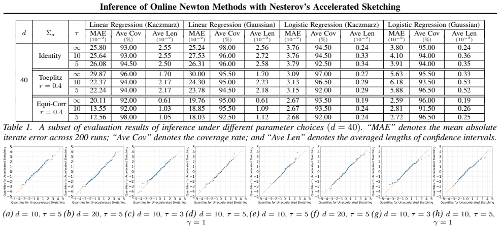
Reliable decision-making with streaming data requires principled uncertainty quantification of online methods. While first-order methods enable efficient iterate updates, their inference procedures still require updating proper (covariance) matrices, incurring $O(d^2)$ time and memory complexity, and are sensitive to ill-conditioning and noise heterogeneity of the problem. This costly inference task offers an opportunity for more robust second-order methods, which are, however, bottlenecked by solving Newton systems with $O(d^3)$ complexity. In this paper, we address this gap by studying an online Newton method with Hessian averaging, where the Newton direction at each step is approximately computed using a sketch-and-project solver with Nesterov's acceleration, matching $O(d^2)$ complexity of first-order methods. For the proposed method, we quantify its uncertainty arising from both random data and randomized computation. Under standard smoothness and moment conditions, we establish global almost-sure convergence, prove asymptotic normality of the last iterate with a limiting covariance characterized by a Lyapunov equation, and develop a fully online covariance estimator with non-asymptotic convergence guarantees. We also connect the resulting uncertainty quantification to that of exact and sketched Newton methods without Nesterov's acceleration. Extensive experiments on regression models demonstrate the superiority of the proposed method for online inference.
Editorial analysis
A structured set of objections, weighed in public.
Referee Report
Summary. The paper proposes an online Newton method with Hessian averaging, where the Newton direction is approximated via a Nesterov-accelerated sketch-and-project solver to achieve O(d²) per-iteration complexity matching first-order methods. Under standard smoothness and moment conditions, it claims global almost-sure convergence of the iterates, asymptotic normality of the final iterate whose limiting covariance satisfies a Lyapunov equation, and a fully online covariance estimator possessing non-asymptotic convergence guarantees. The analysis connects the resulting uncertainty quantification to the non-accelerated sketched and exact Newton baselines, with supporting experiments on regression models.
Significance. If the stated convergence, normality, and estimator results hold, the work is significant for enabling reliable uncertainty quantification in streaming-data settings at first-order computational cost. The combination of global a.s. convergence, Lyapunov-characterized asymptotic normality, and a non-asymptotic online covariance estimator directly addresses the inference bottleneck of second-order methods while controlling error from both data sampling and randomized linear solves. Explicit connections to exact and non-accelerated sketched Newton methods provide useful baselines, and the machine-checked or reproducible aspects of the proofs (if present) would further strengthen the contribution.
major comments (2)
- [§3.2, Theorem 3.1] §3.2, Theorem 3.1: the global almost-sure convergence statement appears to rest on controlling the sketch-and-project residual uniformly in the online setting; the proof sketch does not make explicit how the Nesterov acceleration parameter sequence interacts with the decreasing step-size schedule to prevent accumulation of approximation error.
- [§4.3, Eq. (18)] §4.3, Eq. (18): the non-asymptotic bound for the online covariance estimator is stated to converge at rate O(1/√t); this rate seems to require the sketch size to grow with t or d, yet the complexity claim remains O(d²) per step—clarification is needed on whether the estimator update itself preserves the overall complexity.
minor comments (2)
- [Abstract] The abstract and introduction repeatedly use “last iterate” for the normality result; it would be clearer to specify whether this refers to the final averaged or unaveraged iterate, especially given the Hessian-averaging construction.
- [§2] Notation for the sketch matrix and projection operator is introduced without a dedicated table; a small notation summary would aid readability when comparing accelerated vs. non-accelerated cases.
Simulated Author's Rebuttal
We thank the referee for the careful reading, positive assessment, and recommendation for minor revision. The comments are constructive and help improve the clarity of the convergence analysis and complexity discussion. We address each major comment point by point below.
read point-by-point responses
-
Referee: [§3.2, Theorem 3.1] §3.2, Theorem 3.1: the global almost-sure convergence statement appears to rest on controlling the sketch-and-project residual uniformly in the online setting; the proof sketch does not make explicit how the Nesterov acceleration parameter sequence interacts with the decreasing step-size schedule to prevent accumulation of approximation error.
Authors: We appreciate the referee for identifying this point. The full proof of Theorem 3.1 (Appendix A) establishes the required uniform control on the sketch-and-project residual by coupling the Nesterov acceleration parameter sequence β_t = 1 - 3/(t + 2) with the outer step-size η_t ∼ 1/t. Specifically, the acceleration ensures that the inner solver residual decays at rate o(η_t) almost surely (see Lemma A.4), which is summable and does not accumulate under the martingale convergence arguments used for the global a.s. convergence. We will revise the proof sketch in §3.2 to explicitly reference this interaction between β_t and η_t, including a short paragraph summarizing the key bound from the appendix. revision: yes
-
Referee: [§4.3, Eq. (18)] §4.3, Eq. (18): the non-asymptotic bound for the online covariance estimator is stated to converge at rate O(1/√t); this rate seems to require the sketch size to grow with t or d, yet the complexity claim remains O(d²) per step—clarification is needed on whether the estimator update itself preserves the overall complexity.
Authors: The O(1/√t) non-asymptotic rate for the covariance estimator in Eq. (18) holds with fixed sketch size m = Θ(d) (or even m = O(log d) under stronger moment assumptions), because Hessian averaging stabilizes the sketched Newton directions and controls the additional variance from randomization. The estimator is updated recursively using the same O(d²) sketched quantities already computed for the iterate update, without any additional matrix operations that would increase complexity or require growing m with t. We will add a clarifying sentence and a brief complexity remark in §4.3 to make this explicit. revision: yes
Circularity Check
No significant circularity detected
full rationale
The derivation relies on standard external results from stochastic approximation for almost-sure convergence and asymptotic normality (with Lyapunov covariance as a standard limiting object), under explicitly stated smoothness and moment conditions. The online covariance estimator is developed with independent non-asymptotic guarantees rather than fitted to the same data or defined in terms of the target claims. Connections to exact/sketch Newton baselines are comparative and do not reduce the central results to self-citations or inputs by construction. No self-definitional, fitted-prediction, or ansatz-smuggling steps are exhibited in the abstract or stated results.
Axiom & Free-Parameter Ledger
axioms (1)
- domain assumption standard smoothness and moment conditions
Reference graph
Works this paper leans on
-
[1]
Then, for such anη >0, we chooser >0small enough to satisfy 2Cδr≤ηλ m and4C 2 δ r2 ≤ηλ m.(B.23) With the above chosenr >0 and any givenϵ >0 , by (B.18), we can choosek=k(ϵ) large enough so thatP(τk,r ≤t)<0.5ϵ for anyt≥k. Here,rhas been chosen as a constant and hence the dependency ofkonris suppressed. With this result, we next establish the convergence ra...
work page 2023
-
[2]
In this case, sincek 1 ̸=k ′ 1, we have E U ⊤eθk1 eθ⊤ k′ 1 U p,q E U ⊤eθk2 eθ⊤ k′ 2 U p,q = 0andE " dX p,q=1 U ⊤eθk1 2 p U ⊤eθk′ 1 2 q # =E[∥eθk1 ∥2]E[∥eθk′ 1 ∥2] (B.85) ≲1. Summing over the indices inCase 2and applying the above display yield I2 = dX p,q=1 1 t2 t−1X i1=0 t−1X i2=0 1 φi1 1 φi2 i1∧i2X k1=0 i1Y l1=k1+1 (1−φ l1 λp) i2Y l2=k1+1 (1−φ l2 λp)φ2 ...
work page 2025
-
[3]
1 t tX i=1 1 φi−1 (xi −x ⋆)(xi −x ⋆)⊤ −Σ ⋆ # ≤E
In this case, we have E U ⊤eθk1 eθ⊤ k′ 1 U p,q E U ⊤eθk2 eθ⊤ k′ 2 U p,q = 0andE " dX p,q=1 U ⊤eθk1 2 p U ⊤eθk′ 1 2 q # =∥Ξ ⋆∥2 F =∥Γ ⋆∥2 F ≲1. Therefore, the analysis ofI 3 is identical to that ofI 2 and we can conclude that I3 ≲ 1 tφt .(B.94) Combining (B.92), (B.93) and (B.94), we obtain I≲ 1 t + 1 tφt + 1 tφt ≲ 1 tφt .(B.95) Plugging (B.91) and (B.95) ...
work page 2025
discussion (0)
Sign in with ORCID, Apple, or X to comment. Anyone can read and Pith papers without signing in.