An End-to-End PyTorch Interface for Differentiable PDE Solvers: A RANS Model-Correction Study
Pith reviewed 2026-06-30 17:50 UTC · model grok-4.3
The pith
Reformulating a differentiable PDE solver as an implicit PyTorch layer lets users add and optimize a trainable correction term for inverse problems such as RANS closure modeling.
A machine-rendered reading of the paper's core claim, the machinery that carries it, and where it could break.
Core claim
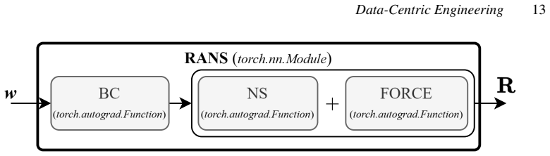
By writing the corrected residual as R(w) + f_phi(w) = 0 and solving it as an implicit layer, the parameters phi of the correction can be optimized directly inside arbitrary PyTorch loss functions; the baseline solver supplies the state w and the autograd graph propagates gradients through the nonlinear solve without manual derivation or finite differences. The method is shown to work for both scalar parameter fitting and full-field neural-network corrections on the RANS equations.
What carries the argument
The implicit-layer reformulation of the residual equation R(w) = 0 together with an additive differentiable correction f_phi(w), which lets PyTorch autograd flow through the solver.
If this is right
- The same interface can be used for data assimilation by optimizing parameters to match observed flow fields.
- Turbulence closure terms or portions of them can be replaced by neural networks whose weights are trained inside the solver loop.
- The workflow extends directly to other physics-informed inverse problems that combine PDE residuals with trainable components.
- Spatial fields such as eddy viscosity can be reconstructed by treating their values at mesh points as trainable parameters.
Where Pith is reading between the lines
- The approach could replace custom adjoint implementations in many engineering optimization loops if the baseline solver is already available in differentiable form.
- Integration into larger machine-learning pipelines would allow joint training of geometry parameters, boundary conditions, and closure models in one graph.
- The method might be tested on other equation types such as heat conduction or linear elasticity to check whether the implicit-layer trick remains stable.
Load-bearing premise
The baseline PDE solver must already be fully differentiable with respect to its inputs and parameters.
What would settle it
Run the framework on a simple Poisson equation whose exact solution is known, add a deliberately incorrect correction term, and check whether the optimizer can recover the correct phi values to within a small tolerance.
Figures

read the original abstract
This work presents an end-to-end strategy for solving inverse problems constrained by Partial Differential Equations within a fully differentiable Machine Learning framework. The proposed formulation provides a unified and user-friendly methodology applicable to a wide range of problems, from data assimilation to closure modeling. Our approach combines a baseline differentiable PDE solver, which predicts the state w from the nonlinear system $R(w) = 0$, with a generic additive, parametrized, and differentiable correction $f_\phi(w)$, with trainable parameters $\phi$. We show how to optimize phi within a fully differentiable Python workflow by reformulating the PDE as an implicit layer, enabling its integration into arbitrary objective functions, while leveraging PyTorch's automatic differentiation graph. The method is demonstrated on the Reynolds-Averaged Navier-Stokes equations for compressible flows, where the closure term, or a portion of it, is modeled using trainable parameters or a Neural Network. The first application considers the 2D NASA Wall-Mounted Hump test case, where a production-term parameter is optimized against time-averaged LES data. A second application is carried out on the VKI LS-59 turbine blade, where the Spalart-Allmaras eddy viscosity field is reconstructed through the optimization of a trainable spatial field. A dataset is generated starting from the VKI LS-59 turbine blade geometry using the differentiable BROADCAST solver with the Spalart-Allmaras turbulence model. The results highlight the flexibility of the framework, showing its applicability beyond turbulence modeling to a broader class of physics-informed PDE-constrained problems with data-driven components.
Editorial analysis
A structured set of objections, weighed in public.
Referee Report
Summary. The manuscript presents an end-to-end PyTorch framework that reformulates a differentiable PDE solver as an implicit layer to enable gradient-based optimization of an additive correction term f_φ(w) for the residual R(w)=0. This is applied to RANS turbulence modeling, with two demonstrations: optimization of a production-term parameter in the NASA Wall-Mounted Hump case against time-averaged LES data, and reconstruction of the Spalart-Allmaras eddy viscosity field on the VKI LS-59 turbine blade using the BROADCAST solver. The approach is positioned as a unified interface for data assimilation and closure modeling problems.
Significance. If the quantitative results support the claims, the work offers a practical, user-friendly interface for embedding existing differentiable PDE solvers into PyTorch workflows via implicit layers. This could lower the barrier for physics-informed inverse problems in CFD without requiring custom adjoint derivations, and the two RANS examples illustrate applicability to parameter fitting and field reconstruction.
major comments (2)
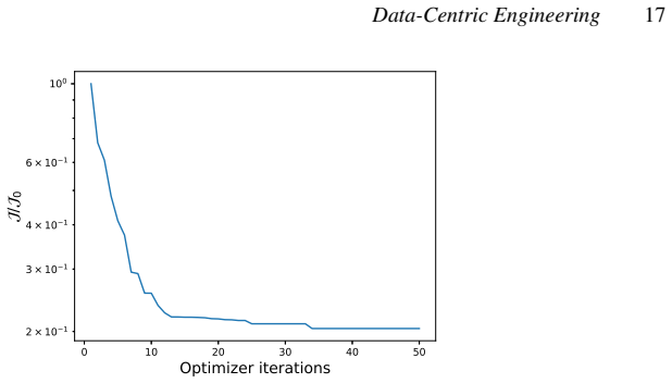
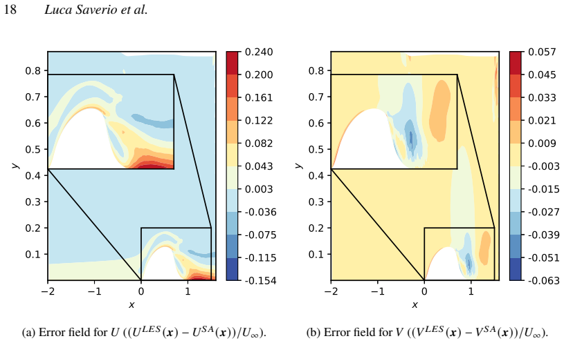
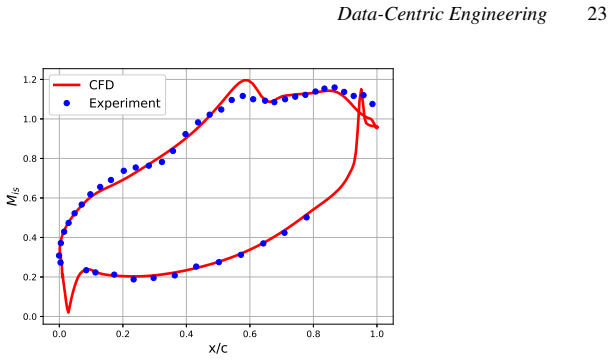
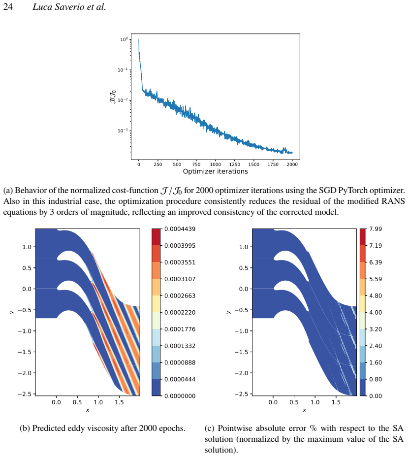
- [Abstract / Results] Abstract and results sections: The demonstrations on the NASA hump and VKI LS-59 cases are described as successful, but the provided text supplies no quantitative error metrics (e.g., L2 norms, drag/lift errors), convergence histories, or ablation studies comparing corrected vs. baseline solutions. This information is load-bearing for the central claim that the implicit-layer formulation enables effective model correction.
- [Method / Implicit Layer] Implicit layer construction (around Eq. for R(w)=0): The formulation assumes the baseline solver (BROADCAST) is fully differentiable w.r.t. inputs and parameters so that gradients flow through the nonlinear solve without finite differences. The manuscript should explicitly verify this property holds for the compressible RANS system with the Spalart-Allmaras model in the two test cases, as it is a prerequisite for the end-to-end claim.
minor comments (2)
- [Abstract] Notation: The correction is introduced as both f_φ(w) and a 'trainable spatial field' in the VKI case; a single consistent symbol and a brief statement of how the spatial field is parametrized would improve clarity.
- [Abstract / Conclusions] The claim of applicability 'to a broader class of physics-informed PDE-constrained problems' is stated but not supported by any non-RANS example; either qualify the statement or move it to future work.
Simulated Author's Rebuttal
We thank the referee for the constructive review and for recognizing the potential of the proposed PyTorch interface. We address each major comment below and indicate the corresponding revisions.
read point-by-point responses
-
Referee: [Abstract / Results] Abstract and results sections: The demonstrations on the NASA hump and VKI LS-59 cases are described as successful, but the provided text supplies no quantitative error metrics (e.g., L2 norms, drag/lift errors), convergence histories, or ablation studies comparing corrected vs. baseline solutions. This information is load-bearing for the central claim that the implicit-layer formulation enables effective model correction.
Authors: We agree that quantitative metrics are essential to substantiate the claims. The revised manuscript adds L2-norm errors on velocity and pressure, drag and lift coefficient errors for the hump case, optimization convergence histories, and direct baseline-versus-corrected comparisons (including an ablation on the correction term) to both the abstract and a dedicated results subsection. These additions are supported by the existing data generated with the BROADCAST solver. revision: yes
-
Referee: [Method / Implicit Layer] Implicit layer construction (around Eq. for R(w)=0): The formulation assumes the baseline solver (BROADCAST) is fully differentiable w.r.t. inputs and parameters so that gradients flow through the nonlinear solve without finite differences. The manuscript should explicitly verify this property holds for the compressible RANS system with the Spalart-Allmaras model in the two test cases, as it is a prerequisite for the end-to-end claim.
Authors: BROADCAST implements the compressible RANS equations with the Spalart-Allmaras model using a fully differentiable residual evaluation, so that the implicit-layer formulation propagates exact gradients via automatic differentiation. To make this explicit, the revised methods section now includes a verification subsection that compares implicit-layer gradients against central finite differences for small perturbations of the production parameter (hump) and the eddy-viscosity field (VKI blade), confirming agreement within numerical tolerance for both cases. revision: yes
Circularity Check
No circularity: framework demonstration relies on external differentiability and intended data-fitting use case
full rationale
The paper presents a software interface that wraps an existing differentiable PDE solver (BROADCAST) as a PyTorch implicit layer to enable gradient-based optimization of an additive correction term f_φ(w) for inverse RANS problems. The two demonstrations optimize a production-term parameter against LES data and reconstruct an eddy-viscosity field; both are explicit inverse-problem fits to supplied data, which is the stated purpose rather than an out-of-sample prediction. No equation or claim reduces by construction to its own inputs, no uniqueness theorem is invoked, and no self-citation chain is load-bearing for the central methodology. The derivation is self-contained once the baseline solver's differentiability is granted externally.
Axiom & Free-Parameter Ledger
free parameters (1)
- phi
axioms (1)
- domain assumption The baseline PDE solver that computes w from R(w)=0 is differentiable with respect to its inputs and parameters.
Reference graph
Works this paper leans on
-
[1]
Journal of Applied Fluid Mechanics 17(12), 2514–2532
Aly AM (2024) Deep Learning-Based Eddy Viscosity Modeling for Improved RANS Simulations of Wind Pressures on Bluff Bodies. Journal of Applied Fluid Mechanics 17(12), 2514–2532. ISSN: 1735-3572. doi: 10.47176/jafm.17.12.2770 . eprint: https://www.jafmonline.net/article_2512_f958e5979d404a47b904e6f736c36eed.pdf . https://www.jafmonline.net/article_ 2512.htm...
-
[2]
ACM Transactions on Mathematical Software 45 (1), 2:1–2:26
Performance and Scalability of the Block Low-Rank Multifrontal Factorization on Multicore Architectures. ACM Transactions on Mathematical Software 45 (1), 2:1–2:26. Amestoy P, Duff IS, Koster J and L’Excellent JY(2001) A Fully Asynchronous Multifrontal Solver Using Distributed Dynamic Scheduling. SIAM Journal on Matrix Analysis and Applications 23(1), 15–...
2001
-
[3]
https: //doi.org/10.21105/joss.07602
doi: 10.21105/joss.07602 . https: //doi.org/10.21105/joss.07602. Bai S, Kolter JZ and Koltun V (2019) Deep equilibrium models. Advances in Neural Information Processing Systems
-
[4]
In 16th aerospace sciences meeting,
Baldwin B and Lomax H (1978) Thin-layer approximation and algebraic model for separated turbulentflows. In 16th aerospace sciences meeting,
1978
-
[5]
Berahas AS and Takáč M (2019) A Robust Multi-Batch L-BFGS Method for Machine Learning. arXiv: 1707.08552 [math.OC]. Available at https://arxiv.org/abs/1707.08552. Boussinesq J (1877) Essai sur la théorie des eaux courantes. Mémoires présentés par divers savants, Paris, France: Académie des Sciences, 1–680. Brantner B, Romemont G de, Kraus M and Li Z (2024...
-
[6]
doi: 10.3389/fphy.2024.1347657. Chu M and Qian W (2024) Physics Constrained Deep Learning For Turbulence Model Uncertainty Quantification . arXiv: 2405.16554 [physics.flu-dyn]. Available at https://arxiv.org/abs/2405.16554. REFERENCES 31 Cinnella P and Content C (2016) High-order implicit residual smoothing time scheme for direct and large eddy simulation...
-
[7]
In ASME-JSME-KSME 2011 Joint Fluids Engineering Conference, AJK
Robust shape optimization of uncertain dense gas flows through a plane turbine cascade. In ASME-JSME-KSME 2011 Joint Fluids Engineering Conference, AJK
2011
-
[8]
Huang K (2008) Statistical Mechanics, 2nd Ed
doi: 10.1115/AJK2011- 05007. Huang K (2008) Statistical Mechanics, 2nd Ed . Wiley India Pvt. Limited. ISBN: 9788126518494. Available at https: // books. google.fr/books?id=ZHl8HLk-K3AC. Jagodzińska I, Olszański B, Gumowski K and Kubacki S (2024) Experimental investigation of subsonic and transonic flows through a linear turbine cascade. European Journal o...
-
[9]
ISSN: 0021-9991. doi: https://doi.org/10.1016/j.jcp.2018.10.045 . https://www.sciencedirect.com/science/article/pii/ S0021999118307125 . Romémont G de, Renac F, Chinesta F, Nunez J and Gueyffier D (2025) Data-Driven Adaptive Gradient Recovery for Unstructured Finite Volume Computations. arXiv: 2507.16571 [math.NA]. Available at https://arxiv.org/abs/2507.1...
-
[10]
Available at https://arxiv.org/abs/2412.07541
07541 [math.NA]. Available at https://arxiv.org/abs/2412.07541. Ruder S (2016) An overview of gradient descent optimization algorithms. arXiv preprint arXiv:1609.04747. Rumsey NC (2020) The Spalart-Allmaras Turbulence Model. https://turbmodels.larc.nasa.gov/spalart.html. Accessed: 2023-07-
-
[11]
SIAM Journal on Scientific and Statistical Computing 7(3), 856–869
Saad Y and Schultz MH (1986) GMRES: A Generalized Minimal Residual Algorithm for Solving Nonsymmetric Linear Sys- tems. SIAM Journal on Scientific and Statistical Computing 7(3), 856–869. doi: 10.1137/0907058. eprint: https://doi.org/10. 1137/0907058. https://doi.org/10.1137/0907058. Sanhueza RD, Smit S, Peeters J and Pecnik R (2022) Machine Learning for ...
-
[12]
Theoretical and Applied Mechanics Letters 11 (4)
End-to-end differentiable learning of turbulence models from indirect observations. Theoretical and Applied Mechanics Letters 11 (4). ISSN: 20950349. doi: 10.1016/j.taml.2021.100280. Talagrand O (1997) Assimilation of observations, an introduction. Journal of the Meteorological Society of Japan 75(1B), 191–
-
[13]
Tankaria H, Sugimoto S and Yamashita N(2021) A Regularized Limited Memory BFGS method for Large-Scale Unconstrained Optimization and its Efficient Implementations. arXiv: 2101.04413 [math.OC]. Available athttps://arxiv.org/abs/2101.04413. Torquato S et al (2002) Random heterogeneous materials: microstructure and macroscopic properties. vol
-
[14]
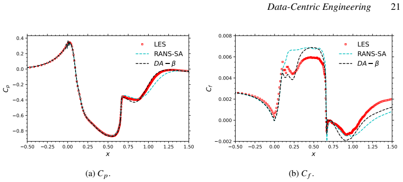
Springer. Uzun A and Malik MR (2018) Large-Eddy Simulation of Flow over a Wall-Mounted Hump with Separation and Reattachment. AIAA Journal 56(2), 715–730. doi: 10.2514/1.J056397. eprint: https://doi.org/10.2514/1.J056397. https://doi.org/10.2514/1. J056397. Wilcox D (2006) Turbulence Modeling for CFD, 3rd ed. DCW Industries. Wu JL, Xiao H and Paterson E (3
-
[15]
Physics-informed machine learning approach for augmenting turbulence models: A comprehensive framework. Physical Review Fluids 7 (3). ISSN: 2469990X. doi: 10.1103/PhysRevFluids.3.074602. Zhang XL, Xiao H, Jee S and He G (2023) Physical interpretation of neural network-based nonlinear eddy viscosity models. Aerospace Science and Technology 142, 108632. ISS...
-
[16]
saved_tensors 12 x_sol , parameters = saved 13 JT = ctx.JT 14 grad_x = ADJOINT_solver (JT , grad_output ) 15 f = F(x_sol , parameters ) 16 grads_params = torch
8 return x_sol 9 @staticmethod 10 def backward (ctx , grad_output ): 11 saved = ctx. saved_tensors 12 x_sol , parameters = saved 13 JT = ctx.JT 14 grad_x = ADJOINT_solver (JT , grad_output ) 15 f = F(x_sol , parameters ) 16 grads_params = torch . autograd . grad ( outputs =f, inputs = parameters , grad_outputs = grad_x ) 17 return grad_x , grads_params , ...
1901
discussion (0)
Sign in with ORCID, Apple, or X to comment. Anyone can read and Pith papers without signing in.