Pathologist-Level Grading of Prostate Biopsies with Artificial Intelligence
Pith reviewed 2026-05-25 11:10 UTC · model grok-4.3
The pith
Deep neural networks detect and grade prostate cancer in needle biopsies at the level of expert pathologists.
A machine-rendered reading of the paper's core claim, the machinery that carries it, and where it could break.
Core claim
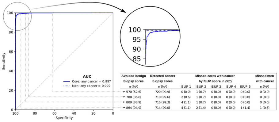
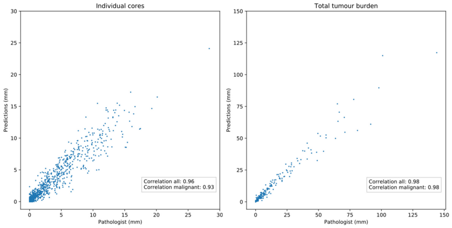
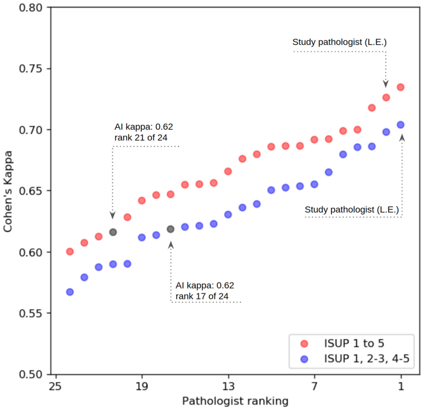
Deep neural networks trained on digitized prostate needle biopsies achieve performance comparable to that of 23 experienced urological pathologists when detecting cancer, estimating its extent, and assigning Gleason grades, as quantified by ROC analysis, millimeter-length correlation, and Cohen's kappa on an independent test set.
What carries the argument
Deep neural networks that classify whole-slide images of prostate needle biopsies for the presence, millimeter extent, and Gleason grade of malignant tissue.
If this is right
- The AI could assist pathology departments facing rising biopsy volumes and a shortage of uro-pathologists.
- Consistent AI grading could reduce intra- and inter-observer variability that currently contributes to over- and undertreatment.
- The method's high discrimination between men with and without cancer suggests utility in both diagnostic and screening contexts.
- The networks' agreement with experts on cancer length and grade indicates they could serve as a stable reference standard.
Where Pith is reading between the lines
- Integration into clinical workflows could let pathologists focus review time on the most ambiguous or borderline cases.
- The same image-classification approach could be tested on other biopsy types where grading variability affects treatment decisions.
- Outcome-linked studies could check whether AI-assisted grading changes rates of progression or survival compared with current expert-only practice.
Load-bearing premise
The grades assigned by the original reporting pathologist and the 23 ISUP experts constitute reliable ground truth.
What would settle it
A fresh panel of pathologists independently re-grading the same 1,631 test biopsies and producing an average pairwise kappa for the AI that falls below the range achieved by those pathologists.
Figures
read the original abstract
Background: An increasing volume of prostate biopsies and a world-wide shortage of uro-pathologists puts a strain on pathology departments. Additionally, the high intra- and inter-observer variability in grading can result in over- and undertreatment of prostate cancer. Artificial intelligence (AI) methods may alleviate these problems by assisting pathologists to reduce workload and harmonize grading. Methods: We digitized 6,682 needle biopsies from 976 participants in the population based STHLM3 diagnostic study to train deep neural networks for assessing prostate biopsies. The networks were evaluated by predicting the presence, extent, and Gleason grade of malignant tissue for an independent test set comprising 1,631 biopsies from 245 men. We additionally evaluated grading performance on 87 biopsies individually graded by 23 experienced urological pathologists from the International Society of Urological Pathology. We assessed discriminatory performance by receiver operating characteristics (ROC) and tumor extent predictions by correlating predicted millimeter cancer length against measurements by the reporting pathologist. We quantified the concordance between grades assigned by the AI and the expert urological pathologists using Cohen's kappa. Results: The performance of the AI to detect and grade cancer in prostate needle biopsy samples was comparable to that of international experts in prostate pathology. The AI achieved an area under the ROC curve of 0.997 for distinguishing between benign and malignant biopsy cores, and 0.999 for distinguishing between men with or without prostate cancer. The correlation between millimeter cancer predicted by the AI and assigned by the reporting pathologist was 0.96. For assigning Gleason grades, the AI achieved an average pairwise kappa of 0.62. This was within the range of the corresponding values for the expert pathologists (0.60 to 0.73).
Editorial analysis
A structured set of objections, weighed in public.
Referee Report
Summary. The paper claims that deep neural networks trained on 6,682 digitized prostate needle biopsies from the STHLM3 study can detect and grade cancer at pathologist-level performance. On an independent test set of 1,631 biopsies, the model achieves AUC 0.997 for benign vs. malignant cores, AUC 0.999 for cancer presence per patient, and 0.96 correlation for millimeter cancer length. On a separate set of 87 biopsies graded by 23 ISUP experts, the AI attains an average pairwise kappa of 0.62, which lies within the experts' inter-rater range of 0.60–0.73.
Significance. If the results hold, this constitutes a meaningful demonstration that AI can match expert urological pathologists on a clinically important task with known high variability and workforce constraints. The work is strengthened by its use of a large population-based training cohort, clear reporting of AUC/correlation/kappa metrics on held-out data, and direct multi-expert comparison panel; these elements provide concrete, falsifiable performance numbers that support potential utility for workload reduction and grading harmonization.
major comments (2)
- [Methods] Methods (training and evaluation protocol): The networks are trained exclusively on labels from the original reporting pathologist (6,682 biopsies). The AUCs of 0.997/0.999 on the 1,631-biopsy test set are therefore measured against this single labeling source. Because Gleason grading exhibits substantial inter-observer variability, this choice makes the ground-truth assumption load-bearing for interpreting the metrics as evidence of expert-level capability rather than successful replication of one particular labeling distribution; the manuscript should discuss or bound the effect of training-label noise on the reported performance.
- [Results] Results (expert panel): The key evidence for the 'pathologist-level' claim is the average pairwise kappa of 0.62 on the 87 biopsies graded by 23 experts, stated to fall within the experts' own range (0.60–0.73). The manuscript must explicitly confirm that these 87 biopsies were strictly excluded from both the 6,682 training biopsies and the 1,631 test set; any overlap would render the kappa comparison non-independent and weaken the generalization argument.
minor comments (1)
- [Abstract] Abstract and Methods: Additional detail on network architecture, loss functions, data augmentation, and training hyperparameters would improve reproducibility assessment without altering the central claims.
Simulated Author's Rebuttal
We thank the referee for the detailed and constructive comments. We address each major point below and will revise the manuscript accordingly where appropriate.
read point-by-point responses
-
Referee: [Methods] Methods (training and evaluation protocol): The networks are trained exclusively on labels from the original reporting pathologist (6,682 biopsies). The AUCs of 0.997/0.999 on the 1,631-biopsy test set are therefore measured against this single labeling source. Because Gleason grading exhibits substantial inter-observer variability, this choice makes the ground-truth assumption load-bearing for interpreting the metrics as evidence of expert-level capability rather than successful replication of one particular labeling distribution; the manuscript should discuss or bound the effect of training-label noise on the reported performance.
Authors: We agree that training and primary evaluation rely on labels from a single reporting pathologist and that inter-observer variability in Gleason grading is well-documented. The reported AUCs therefore reflect agreement with that specific labeling distribution rather than an absolute ground truth. The primary evidence for pathologist-level performance is the separate multi-expert panel (kappa comparison), which is independent of the original labels. We will add an explicit discussion of label noise and its potential effect on the AUC/correlation metrics in the revised Methods and Discussion sections. revision: yes
-
Referee: [Results] Results (expert panel): The key evidence for the 'pathologist-level' claim is the average pairwise kappa of 0.62 on the 87 biopsies graded by 23 experts, stated to fall within the experts' own range (0.60–0.73). The manuscript must explicitly confirm that these 87 biopsies were strictly excluded from both the 6,682 training biopsies and the 1,631 test set; any overlap would render the kappa comparison non-independent and weaken the generalization argument.
Authors: The 87 biopsies constitute a separate evaluation cohort that was not part of the 6,682 training biopsies or the 1,631-biopsy test set; this is indicated by the phrasing 'additionally evaluated' and 'separate set' in the manuscript. To remove any ambiguity we will add an explicit statement confirming the strict exclusion of these cases from both the training and test sets. revision: yes
Circularity Check
No circularity; metrics from held-out evaluation on external expert labels
full rationale
The paper trains DNNs on original pathologist labels for 6682 biopsies then reports AUC, correlation, and kappa on fully independent test sets (1631 biopsies + 87 expert-graded biopsies). No equations, normalizations, or self-citations reduce any reported metric to quantities fitted on the same data by construction. Evaluation uses external benchmarks (held-out labels and ISUP panel inter-rater kappa), satisfying the self-contained criterion.
Axiom & Free-Parameter Ledger
free parameters (1)
- neural network weights and biases
Reference graph
Works this paper leans on
-
[1]
Sample collection Sample collection was carried out in two rounds. The first selection was the first 500 men with prostate cancer who were diagnosed in the Stockholm - 3 study. All 10 - 12 cores from these men were scanned, in total 5,662 slides. The second round included all m en with at least one core graded as Gleason Score (GS) 4+4 or 5+5 to enrich th...
work page 2016
-
[2]
2.5.86 (Hamamatsu Photonics, Hamamatsu, Japan)
Image acquisition The first round of slides was digitized using a Hamamatsu C9600 - 12 scanner and NDP.scan software v. 2.5.86 (Hamamatsu Photonics, Hamamatsu, Japan). The following batches of slides were scanned using an Aperio ScanScope AT2 scanner and Aperio Image Library v. 12.0.15 software (Leica Biosystems, Wetzlar, Germany). The pixel size at full ...
-
[3]
The GPUs were running Nvidia driver v
Hardware and software Computations were performed on two graphics processing unit (GPU) c lusters (Tampere Center for Scientific Computing, Finland and CSC IT Center for Science, Finland), utilizing a total of 136 x Tesla P100 GPUs (Nvidia, Santa Clara, CA, USA), distributed on 37 nodes. The GPUs were running Nvidia driver v. 410.79, CUDA v. 9. 2.148 and ...
-
[4]
Segmentation of tissue Our image pre - processing wo rkflow is depicted in Figure S1
Image pre - processing 4.1. Segmentation of tissue Our image pre - processing wo rkflow is depicted in Figure S1 . First, we employed a Laplacian filtering algorithm to separate tissue from background and pen mark annotations. We first read images downsampled by a factor of 16 directly from the resolution pyramids present in the image f iles using Opensli...
work page 2000
-
[5]
That is, instead of assigning a nnotated tissue pixels the label 2 (i.e
The color producing the shortest distance was used as the basis of labeling the corresponding tissue region. That is, instead of assigning a nnotated tissue pixels the label 2 (i.e. cancer) in the label mask L , we assigned the values 3 (Gleason 3), 4 (Gleason 4) or 5 (Gleason 5). Pixels with conflicting labels indicated by multiple, differently colored p...
-
[6]
Data management and quality control Prior to image preprocessing, all WSIs were v isually examined to exclude slides unsuitable for analysis . The excluded slides included 86 slides representing immunohistochemical instead of H&E staining, 8 slides with failed H&E staining resulting in near complete lack of stain , 3 slides with corrupted data, and 23 sli...
-
[7]
Model We used a two - stage model for classifying individual image patches (see Figure S2 )
Patch - level classifier 6.1. Model We used a two - stage model for classifying individual image patches (see Figure S2 ). The first stage of the model classifies image patches in binary fashion as either benign or cancerous, while the second stage performs Gleason grading. We included the benign class also into the second stage model in order to obtain a...
-
[8]
it allowed uncoupling the training of models for the detection and grading tasks, which require different numbers of trai ning epochs to avoid overfitting, and 3) it enables adjusting the classifier’s operating point for the cancer detection task in a straightforward manner, independently of the Gleason grading task (see Section 6.2. for details). We eval...
-
[9]
Slide - level classifier 7.1. Model We employed a model - based approach relying on boosted trees, implemented using XGBoost 16 , for aggregating patch - level predictions into slide - level predictions (see Figure S2 ). We trained one boosted tree classifier based on the patch - level pred ictions of each 29 CNN, thus forming ensembles of boosted trees. ...
-
[10]
Supplementary results 8.1. Model architecture comparison We compared different CNN architectures in terms of their performance based on a single validation split, where a random selec tion of 20% and 80% of the men in training data were allocated for validation and training, respectively (i.e. no data from the test set was used for these experiments) . In...
-
[11]
Supplementary Figures Figure S1: Image pre - processing workflow. (A) From left to right: tissue (blue outline) and annotations drawn with a pen (red outline) are segmented from the input WSI and stored as binary masks. The annotations are then digitized by projecting the pen marks onto adjacent tissue, and the result is st ored as a label mask indicating...
-
[12]
Scanned slides were linked back to clinical data
Supplementary Tables Table S1: Data management workflow and quality control. Scanned slides were linked back to clinical data. We excluded slides with cor rupted filenames, slides that did not pass the visual quality control, slides that were duplicated during scanning and slides that were not consistent with clinical data. N Total scanned slides 10185 Ex...
discussion (0)
Sign in with ORCID, Apple, or X to comment. Anyone can read and Pith papers without signing in.