Physics Informed Extreme Learning Machine (PIELM) -- A rapid method for the numerical solution of partial differential equations
Pith reviewed 2026-05-25 01:09 UTC · model grok-4.3
The pith
PIELM solves linear partial differential equations with accuracy matching or exceeding PINNs by replacing iterative training with an analytical least-squares step.
A machine-rendered reading of the paper's core claim, the machinery that carries it, and where it could break.
Core claim
Physics Informed Extreme Learning Machine (PIELM) is a rapid version of PINNs applicable to stationary and time-dependent linear partial differential equations. By fixing the hidden weights at random values and determining the output weights through a single least-squares minimization of the physics residual, PIELM matches or exceeds the accuracy of PINNs on tested problems. For large domains the distributed DPIELM variant produces results comparable to conventional numerical techniques.
What carries the argument
Physics Informed Extreme Learning Machine (PIELM), in which hidden-layer weights are drawn once at random and the output-layer weights are obtained by direct least-squares solution of the residual loss rather than gradient-based iteration.
If this is right
- PIELM applies directly to both stationary and time-dependent linear PDEs without retraining the hidden layer.
- Accuracy on the tested problems is at least as good as that obtained by full iterative training of PINNs.
- The distributed DPIELM extension produces solutions on large domains that match the accuracy of standard finite-difference or finite-element codes.
- Neural-network PDE solvers become computationally competitive with conventional discretization methods for linear problems.
Where Pith is reading between the lines
- The training-time reduction could make neural PDE methods viable for real-time or many-query settings such as design optimization loops.
- The same fixed-random-weight idea may transfer to other linear operators beyond the PDE residuals shown here.
- Domain decomposition used in DPIELM could be combined with adaptive mesh refinement to further enlarge the solvable domain size.
- For nonlinear PDEs the direct least-squares step would no longer apply, suggesting the need for iterative outer loops around the ELM solve.
Load-bearing premise
That fixing hidden weights randomly and solving only the output weights by least squares is enough to drive the physics residual to a low value for the linear PDEs considered.
What would settle it
A side-by-side run on one of the paper's benchmark linear PDEs in which the maximum pointwise error of the PIELM solution exceeds the PINN error by more than a factor of two.
Figures




read the original abstract
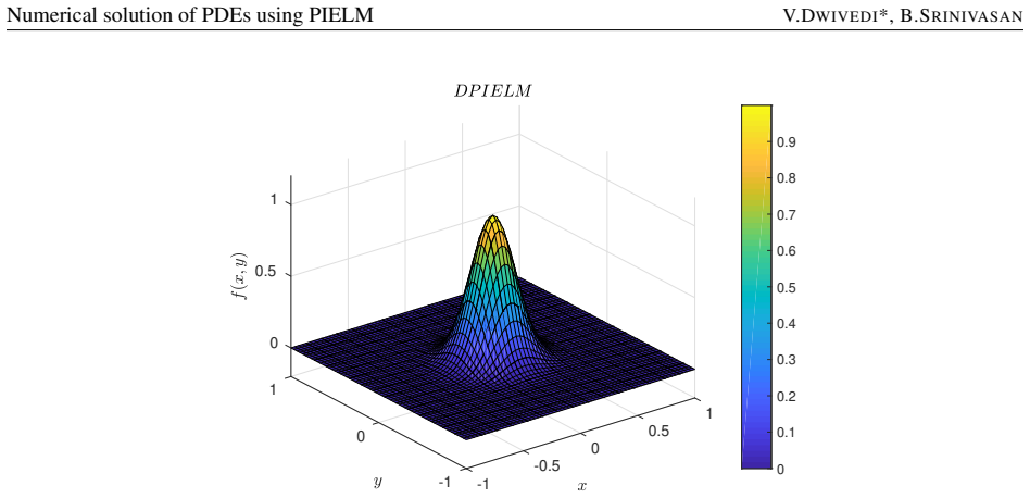
There has been rapid progress recently on the application of deep networks to the solution of partial differential equations, collectively labelled as Physics Informed Neural Networks (PINNs). In this paper, we develop Physics Informed Extreme Learning Machine (PIELM), a rapid version of PINNs which can be applied to stationary and time dependent linear partial differential equations. We demonstrate that PIELM matches or exceeds the accuracy of PINNs on a range of problems. We also discuss the limitations of neural network based approaches, including our PIELM, in the solution of PDEs on large domains and suggest an extension, a distributed version of our algorithm -{}- DPIELM. We show that DPIELM produces excellent results comparable to conventional numerical techniques in the solution of time-dependent problems. Collectively, this work contributes towards making the use of neural networks in the solution of partial differential equations in complex domains as a competitive alternative to conventional discretization techniques.
Editorial analysis
A structured set of objections, weighed in public.
Referee Report
Summary. The manuscript proposes Physics Informed Extreme Learning Machine (PIELM) as a non-iterative variant of Physics Informed Neural Networks (PINNs) for stationary and time-dependent linear PDEs. Hidden-layer weights are drawn randomly and held fixed while output weights are obtained by solving a linear least-squares problem that enforces the PDE residual at collocation points. The authors assert that PIELM matches or exceeds PINN accuracy on a range of problems and introduce a distributed variant (DPIELM) whose results on time-dependent problems are comparable to conventional discretizations. The work also notes scalability limitations of neural approaches on large domains.
Significance. If the empirical demonstrations are robust, PIELM would supply a computationally lighter alternative to gradient-based PINNs for linear problems by replacing iterative optimization with a single linear solve. The distributed extension directly addresses a recognized practical bottleneck. The absence of any theoretical guarantee on the span of the random feature space, however, confines the contribution to an empirical observation whose generality remains to be established.
major comments (2)
- [Abstract] Abstract (paragraph on PIELM development): the central claim that fixed random hidden weights suffice to minimize the physics-informed residual to PINN-level accuracy rests on an unverified empirical property of the random basis; no analysis of the conditioning of the resulting Gram matrix or of the expressivity of the chosen random features is supplied, leaving open the possibility that accuracy holds only for the specific test problems shown.
- [Abstract] Abstract: the statements that PIELM 'matches or exceeds the accuracy of PINNs' and that DPIELM produces 'excellent results comparable to conventional numerical techniques' are presented without reference to quantitative error tables, convergence rates, or domain-size scaling data; such metrics are required to substantiate the load-bearing performance claims.
minor comments (2)
- Notation for the random hidden weights and the collocation-point residual matrix should be introduced explicitly before the least-squares step is described.
- The manuscript should clarify whether the same random-seed protocol is used across all compared methods to ensure fair timing and accuracy comparisons.
Simulated Author's Rebuttal
We thank the referee for the constructive feedback. We address each major comment below, indicating planned revisions to the abstract and manuscript where appropriate.
read point-by-point responses
-
Referee: [Abstract] Abstract (paragraph on PIELM development): the central claim that fixed random hidden weights suffice to minimize the physics-informed residual to PINN-level accuracy rests on an unverified empirical property of the random basis; no analysis of the conditioning of the resulting Gram matrix or of the expressivity of the chosen random features is supplied, leaving open the possibility that accuracy holds only for the specific test problems shown.
Authors: We agree that the work is empirical and supplies no theoretical analysis of Gram-matrix conditioning or random-feature expressivity. The manuscript demonstrates performance on multiple linear PDE test problems but does not claim universality. We will revise the abstract to qualify the central claim as an empirical observation and add a short paragraph in the conclusions acknowledging the absence of such guarantees and the need for future analysis. revision: partial
-
Referee: [Abstract] Abstract: the statements that PIELM 'matches or exceeds the accuracy of PINNs' and that DPIELM produces 'excellent results comparable to conventional numerical techniques' are presented without reference to quantitative error tables, convergence rates, or domain-size scaling data; such metrics are required to substantiate the load-bearing performance claims.
Authors: Detailed quantitative error tables, L2-norm comparisons, and convergence studies appear in Sections 4 and 5 of the manuscript. We will revise the abstract to include explicit numerical error values (e.g., maximum and average L2 errors) and to reference the relevant tables/figures that contain the full data and scaling results. revision: yes
Circularity Check
No circularity: algorithmic proposal with empirical validation only
full rationale
The paper proposes PIELM as a new training procedure (random fixed hidden weights + linear least-squares solve on physics residual) and reports empirical accuracy comparisons to PINNs and conventional solvers on selected linear PDEs. No derivation chain exists that reduces a claimed result to its own inputs by construction; the central assertions are performance statements on tested instances rather than predictions forced by fitted parameters or self-citations. The method is self-contained against external benchmarks (PINN results and standard discretizations) without load-bearing self-referential steps.
Axiom & Free-Parameter Ledger
Lean theorems connected to this paper
-
IndisputableMonolith/Cost/FunctionalEquation.leanwashburn_uniqueness_aczel unclear?
unclearRelation between the paper passage and the cited Recognition theorem.
We have made our ELM “physics informed” by incorporating the information about the physics of PDE as the cost function... Hc = K... pinv(H)K
-
IndisputableMonolith/Foundation/AlexanderDuality.leanalexander_duality_circle_linking unclear?
unclearRelation between the paper passage and the cited Recognition theorem.
PIELM... distributed version... DPIELM... partition into multiple cells
What do these tags mean?
- matches
- The paper's claim is directly supported by a theorem in the formal canon.
- supports
- The theorem supports part of the paper's argument, but the paper may add assumptions or extra steps.
- extends
- The paper goes beyond the formal theorem; the theorem is a base layer rather than the whole result.
- uses
- The paper appears to rely on the theorem as machinery.
- contradicts
- The paper's claim conflicts with a theorem or certificate in the canon.
- unclear
- Pith found a possible connection, but the passage is too broad, indirect, or ambiguous to say the theorem truly supports the claim.
Reference graph
Works this paper leans on
-
[1]
An introduction to computational fluid dynamics: the finite volume method
Versteeg, Henk Kaarle, and Weeratunge Malalasekera. An introduction to computational fluid dynamics: the finite volume method. Pearson education, 2007
work page 2007
-
[2]
A contribution to the great Riemann solver debate
Quirk, James J. " A contribution to the great Riemann solver debate." Upwind and High-Resolution Schemes. Springer, Berlin, Heidelberg, 1997. 550-569
work page 1997
-
[3]
Berg, Jens, and Kaj Nyström. A unified deep artificial neural network approach to partial differential equations in complex geometries. Neurocomputing 317 (2018): 28-41
work page 2018
-
[4]
Artificial neural networks for solving ordinary and partial differential equations
Lagaris, Isaac E., Aristidis Likas, and Dimitrios I. Fotiadis. " Artificial neural networks for solving ordinary and partial differential equations." IEEE transactions on neural networks 9.5 (1998): 987-1000
work page 1998
-
[5]
Neural-network methods for boundary value problems with irregular boundaries
Lagaris, Isaac E., Aristidis C. Likas, and Dimitris G. Papageorgiou. " Neural-network methods for boundary value problems with irregular boundaries." IEEE Transactions on Neural Networks 11.5 (2000): 1041-1049. 28 Numerical solution of PDEs using PIELM V.DWIVEDI *, B.S RINIVASAN
work page 2000
-
[6]
Neural network differential equation and plasma equilibrium solver
van Milligen, B. Ph, V . Tribaldos, and J. A. Jiménez. " Neural network differential equation and plasma equilibrium solver." Physical review letters 75.20 (1995): 3594
work page 1995
-
[7]
McFall, K. S., & Mahan, J. R. (2009). Artificial neural network method for solution of boundary value problems with exact satisfaction of arbitrary boundary conditions. IEEE Transactions on Neural Networks, 20(8), 1221-1233
work page 2009
-
[8]
Kumar, Manoj, and Neha Yadav. "Multilayer perceptrons and radial basis function neural network methods for the solution of differential equations: a survey." Computers & Mathematics with Applications 62.10 (2011): 3796-3811
work page 2011
-
[9]
Application of Legendre Neural Network for solving ordinary differential equations
Mall, Susmita, and Snehashish Chakraverty. " Application of Legendre Neural Network for solving ordinary differential equations." Applied Soft Computing 43 (2016): 347-356
work page 2016
-
[10]
DGM: A deep learning algorithm for solving partial differential equations
Sirignano, Justin, and Konstantinos Spiliopoulos. " DGM: A deep learning algorithm for solving partial differential equations." Journal of Computational Physics 375 (2018): 1339-1364
work page 2018
-
[11]
Hidden physics models: Machine learning of nonlinear partial differential equations
Raissi, Maziar, and George Em Karniadakis. " Hidden physics models: Machine learning of nonlinear partial differential equations." Journal of Computational Physics 357 (2018): 125-141
work page 2018
-
[12]
Numerical gaussian processes for time-dependent and nonlinear partial differential equations
Raissi, Maziar, Paris Perdikaris, and George Em Karniadakis. " Numerical gaussian processes for time-dependent and nonlinear partial differential equations." SIAM Journal on Scientific Computing 40.1 (2018): A172-A198
work page 2018
-
[13]
Raissi, Maziar, Paris Perdikaris, and George E. Karniadakis. " Physics-informed neural networks: A deep learning framework for solving forward and inverse problems involving nonlinear partial differential equations." Journal of Computational Physics 378 (2019): 686-707
work page 2019
-
[14]
G.-B. Huang, Q.-Y . Zhu, C.-K. Siew, Extreme learning machine: theory and applications, Neurocomputing 70 (2006) 489–501
work page 2006
-
[15]
Balasundaram, S. " Application of error minimized extreme learning machine for simultaneous learning of a function and its derivatives." Neurocomputing 74.16 (2011): 2511-2519
work page 2011
-
[16]
Yang, Yunlei, Muzhou Hou, and Jianshu Luo. " A novel improved extreme learning machine algorithm in solving ordinary differential equations by Legendre neural network methods." Advances in Difference Equations 2018.1 (2018): 469
work page 2018
-
[17]
Sun, Hongli, et al. " Solving partial differential equation based on Bernstein neural network and extreme learning machine algorithm." Neural Processing Letters (2018): 1-20
work page 2018
- [18]
-
[19]
D. Rumelhart, G. Hintont, R. Williams, Learning representations by backpropagating errors, Nature 323 (6088) (1986) 533–536
work page 1986
-
[20]
Automatic differentiation in machine learning: a survey
Baydin, Atilim Gunes, et al. " Automatic differentiation in machine learning: a survey." Journal of Machine Learning Research 18 (2018): 1-43
work page 2018
-
[21]
Serre, Matrices: Theory and Applications, Springer, New York, 2002
D. Serre, Matrices: Theory and Applications, Springer, New York, 2002
work page 2002
-
[22]
Kopriva, David A., and Gregor J. Gassner. " An energy stable discontinuous Galerkin spectral element discretization for variable coefficient advection problems." SIAM Journal on Scientific Computing 36.4 (2014): A2076-A2099
work page 2014
-
[23]
A high-order discontinuous Galerkin method for unsteady advection–diffusion problems
Borker, Raunak, Charbel Farhat, and Radek Tezaur. "A high-order discontinuous Galerkin method for unsteady advection–diffusion problems." Journal of Computational Physics 332 (2017): 520-537. 29
work page 2017
discussion (0)
Sign in with ORCID, Apple, or X to comment. Anyone can read and Pith papers without signing in.