REVIEW 7 minor 19 references
Photon-weighted barycentric correction and its importance for precise radial velocities
T0 review · 0 major / 7 minor · reviewed 2026-08-14 · deepseek-v4-flash
Pith's one-line read The standard barycentric correction for long exposures leaves a systematic radial-velocity error, sometimes over 1 m/s, because the correction curves with Earth's rotation rather than changing linearly.
desk verdict A clean, useful derivation of the second-order barycentric correction error that deserves referee time; the central claim holds up. read the letter →
The pith
A machine-rendered reading of the paper's core claim, the machinery that carries it, and where it could break.
The reading
What carries the argument
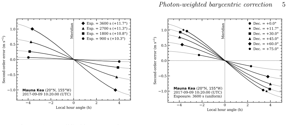
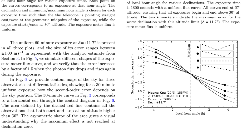
The central object is the photon-weighted average in Equation (3), with the exposure meter flux curve $f(t)$ acting as the smoothing kernel applied to the instantaneous barycentric correction. Expanding $v(t)$ around $\langle t\rangle$ to second order, the missed term is proportional to the time variance of the photon arrival distribution, $\langle t^2\rangle-\langle t\rangle^2$, multiplied by the local curvature $2\pi^2 V_0\sin\psi/(24\,\mathrm{h})^2$; for a uniform exposure the variance becomes $\Delta t^2/12$, producing the compact scaling $\propto \cos(\mathrm{lat})\cos(\delta)\sin\psi\,(\Delta t)^2$ in Equation (10). This machinery turns a correction that is normally a single number into a filter over the exposure, and it predicts that flux curves concentrated at one end shrink the error while curves with a mid-exposure dip grow it.
What would settle it
Take a 60-minute exposure at a low-latitude site on a target with declination near zero observed through the east, record the exposure-meter flux curve, and compare $\langle v\rangle$ computed from the full flux curve with $v(\langle t\rangle)$ computed at the photon-weighted midpoint; the predicted difference is about 1 m/s (scaled by the actual flux shape). A null result at the 10 cm/s level would show the diurnal-curvature model is incomplete.
Extended reading notes
Core claim
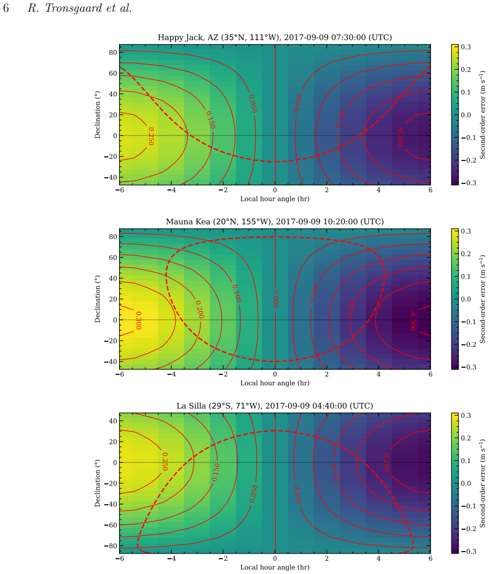
At the center of the paper is the difference between two averages of the barycentric-corrected velocity over an exposure: the value at the photon-weighted midpoint time, $v(\langle t\rangle)$, and the true photon-weighted average $\langle v\rangle$ from Equation (3). Since the diurnal component of $v_B(t)$ is sinusoidal, evaluating at $\langle t\rangle$ always falls inside the curve's curvature, so the second-order error has a definite sign and scales with $\cos(\mathrm{lat})\cos(\delta)\sin\psi\,(\Delta t)^2$; for a uniform exposure it is about $1.32\,\mathrm{m\,s^{-1}}\cos(\mathrm{lat})\cos(\delta)\sin\psi\,(\Delta t/\mathrm{1\,h})^2$. At a low-latitude observatory the worst case allowed by a 30-degree altitude limit gives 0.25 m/s for a 30-minute exposure and 1.0 m/s for 60 minutes, with a V-shaped flux dip amplifying the effect by about 1.5. Full numerical simulations of the barycentric correction reproduce the analytic scaling, and real exposure-meter data for exposures up to 20 minutes shows the constant-flux approximation recovers the correction to within about 1 cm/s. The paper's conclusion is that instruments aiming at 10 cm/s precision must store the flux curve and apply photon weights to the correction itself.
Load-bearing premise
The paper's error estimates rest on modeling the barycentric velocity over an exposure as a pure diurnal sinusoid with a constant hour-angle rate; everything else in the correction is assumed to curve negligibly over tens of minutes, and the real-data check only reaches 20-minute exposures.
Editorial extensions
If this is right
- Storing the exposure meter flux curve in the raw data makes the barycentric correction reproducible at the 1 cm/s level even for hour-long exposures, independent of weather and guiding changes.
- Without photon weighting, a 30-minute low-latitude exposure near the celestial equator can be wrong by 0.25 m/s, and a 60-minute exposure by 1.0 m/s, in the worst observing geometry.
- For archived data that only has the photon-weighted midpoint time, adding the constant-flux correction term of Equation (10) removes most of the second-order error, and real data out to 20 minutes supports this approximation to about 1 cm/s.
- Observers can reduce the error by scheduling near the meridian, shortening exposures, or choosing high-declination targets; the error is largest for rising or setting targets observed through the east or west.
Reading between the lines
- Beyond the paper's own tests, the same curvature argument should apply to any time-varying correction over an exposure, including the chromatic dependence of the barycentric correction, so instruments that archive only midpoint times may have hidden systematics in other correction terms as well.
- The paper does not quantify survey-level impact, but because the error depends on hour angle, nightly-offset fits will partially absorb it; a testable prediction is that archival RV residuals should show a sinusoidal pattern in hour angle with amplitude growing as $\Delta t^2$.
- One could exploit the opposite sign of the error east and west of the meridian: pairs of observations taken at $\pm$ hour angles would show a symmetric curl if this is the dominant systematic, providing a clean null test.
Signed reviews
Editorial analysis
A structured set of objections, weighed in public.
Referee Report
Summary. This manuscript addresses a systematic error in barycentric corrections for radial-velocity (RV) exposures of finite duration. The authors show that the common practice of evaluating the barycentric correction at the photon-weighted midpoint time of an exposure is exact only if the correction varies linearly with time; because the dominant diurnal component is curved, a residual second-order offset remains between the correction evaluated at the photon-weighted mean time and the flux-weighted mean of the instantaneous corrections. They derive analytic estimates (Eqs. 8-10) from a Taylor expansion of a sinusoidal diurnal model, predict errors of 0.25 m/s for a 30 minute and 1.0 m/s for a 60 minute uniform exposure in a worst-case geometry, verify these scalings with barycorrpy simulations for different exposure times, declinations, flux shapes, and observatory latitudes, and use 1315 EXPRES exposures to show that a uniform-flux approximation captures the second-order error to within about 1 cm/s for exposures shorter than 20 minutes. The paper recommends that instruments record and archive exposure-meter flux curves and, for existing data without flux curves, apply a uniform-flux correction term.
Significance. If correct, this is an important and directly actionable result for the precision-RV community. The central derivation is a parameter-free analytic Taylor expansion with no fitted free parameters, and the resulting coefficient in Eq. (10) and the V-shape enhancement factor of 1.5 are concrete, falsifiable predictions. The analytic results are corroborated by simulations with barycorrpy, a widely used and externally benchmarked package, and by a real-data comparison with EXPRES exposure-meter data. The paper closes a gap left open in earlier barycentric-correction work and gives a practical recommendation for both current and future instruments, which is relevant for the 10 cm/s and 1 m/s RV precision regimes.
minor comments (7)
- [Section 5.2 / Fig. 7] The text reports 1315 EXPRES observations, while the Fig. 7 caption states 1316 observations; please reconcile the count.
- [Section 5.2] The statement that "There is no indication that longer exposure times would change this picture" is stronger than the data support, because Fig. 7 contains no exposure longer than 20 minutes; I suggest softening the wording or adding a simulation for longer exposures.
- [Section 3] Equation (10) is obtained from Eq. (9) via the spherical-trig identity cos(δ)sin(ψ) = -cos(alt)sin(az), but the derivation is relegated to a footnote; stating the identity explicitly in the text would make the derivation easier to verify and reproduce.
- [Section 3] The sentence "If photons are concentrated towards one end of the exposure, the error second-order error decreases" contains a typo; please also state explicitly the sign convention for azimuth so that the signs in Figs. 3 and 6 can be interpreted unambiguously.
- [Section 5.2] The claim that "In our experience, a typical offset is of order 5% of the exposure time" is anecdotal and unreferenced; providing a quantitative justification or a reference would strengthen this part of the mitigation discussion.
- [Section 5.2] Footnote 2 describes a step-function mitigation strategy for data without flux curves, but it does not specify exactly how to implement it; a brief formula would make the recommendation reproducible.
- [Section 3] The derivation in Eq. (4) assumes that non-diurnal contributions to the barycentric velocity have negligible curvature over an exposure, and although the barycorrpy simulations support this, the paper would be more self-contained with an explicit order-of-magnitude bound on the neglected terms.
Circularity Check
No significant circularity found; the central derivation is a parameter-free Taylor expansion against an external physical model and is not fitted to the paper's own outputs.
full rationale
The paper's load-bearing result is Equation (9), obtained by inserting a second-order Taylor expansion of the barycentric velocity, Equation (7), into the photon-weighted average, Equation (3). The first-order term cancels by the definition of the photon-weighted midpoint time in Equation (6), leaving only the curvature term proportional to the variance of the arrival-time distribution. No quantity appearing in the final estimate is fitted from the data it is later used to explain; the coefficient in Equation (10) follows from analytically evaluating the integrals for a uniform flux curve. The barycorrpy simulations are an independent numerical check of the analytic estimate, not an input to it, and although Wright and Eastman are co-authors of barycorrpy, the analytic derivation does not rely on that code. The EXPRES comparison in Figure 7 uses real exposure-meter fluxes to test whether the uniform-flux approximation is adequate; it is a validation exercise rather than a fit, and it does not define the predicted error. Self-citations such as Wright & Eastman (2014) and Blackman et al. (2017) provide context and code references but are not load-bearing for the derivation. No step reduces by construction to its own inputs, so the circularity score is 0.
Assumptions & free parameters
assumptions (5)
- domain assumption Over timescales of hours, barycentric velocity is dominated by Earth's diurnal rotation, Eq. (4).
- domain assumption Hour angle rate is constant at 2π/24h.
- domain assumption Exposure meter flux f(t) is proportional to photon flux in the relevant pixel, Eq. (3).
- domain assumption Results for vmeas = 0 generalize to any vmeas much smaller than c.
- domain assumption Without a flux curve, a uniform flux distribution is the most realistic assumption for archived data.
Cite this review
Pith. "Pith review of Photon-weighted barycentric correction and its importance for precise radial velocities." pith.science (2026). https://pith.science/paper/U5SHOZVW
@misc{pith2026190800991,
  author       = {Pith},
  title        = {Pith review of: Photon-weighted barycentric correction and its importance for precise radial velocities},
  year         = {2026},
  howpublished = {\url{https://pith.science/paper/U5SHOZVW}},
  note         = {Machine review of arXiv:1908.00991}
}
abstract
When applying the barycentric correction to a precise radial velocity measurement, it is common practice to calculate its value only at the photon-weighted midpoint time of the observation instead of integrating over the entire exposure. However, since the barycentric correction does not change linearly with time, this leads to systematic errors in the derived radial velocities. The typical magnitude of this second-order effect is of order 10 cm s$^{-1}$, but it depends on several parameters, e.g. the latitude of the observatory, the position of the target on the sky, and the exposure time. We show that there are realistic observing scenarios, where the errors can amount to more than 1 ms$^{-1}$. We therefore recommend that instruments operating in this regime always record and store the exposure meter flux curve (or a similar measure) to be used as photon-weights for the barycentric correction. In existing data, if the flux curve is no longer available, we argue that second-order errors in the barycentric correction can be mitigated by adding a correction term assuming constant flux.
Figures


Figures from the paper (3 more)

Reference graph
Works this paper leans on
-
[1]
Astropy Collaboration et al., 2013, @doi [ ] 10.1051/0004-6361/201322068 , http://adsabs.harvard.edu/abs/2013A
-
[2]
Blackman R. T., Szymkowiak A. E., Fischer D. A., Jurgenson C. A., 2017, @doi [ ] 10.3847/1538-4357/aa5ead , https://ui.adsabs.harvard.edu/#abs/2017ApJ...837...18B 837, 18
-
[3]
Blackman R. T., Ong J. M. J., Fischer D. A., 2019, @doi [ ] 10.3847/1538-3881/ab24c3 , https://ui.adsabs.harvard.edu/abs/2019AJ....158...40B 158, 40
-
[4]
Cosentino R., et al., 2012, in Ground-based and Airborne Instrumentation for Astronomy IV. p. 84461V, @doi 10.1117/12.925738
-
[5]
Fischer D. A., et al., 2016, @doi [Publications of the Astronomical Society of the Pacific] 10.1088/1538-3873/128/964/066001 , https://ui.adsabs.harvard.edu/#abs/2016PASP..128f6001F 128, 066001
-
[6]
Howard A. W., et al., 2013, @doi [ ] 10.1038/nature12767 , https://ui.adsabs.harvard.edu/\#abs/2013Natur.503..381H 503, 381
-
[7]
D., 2007, @doi [Computing In Science & Engineering] 10.1109/MCSE.2007.55 , 9, 90
Hunter J. D., 2007, @doi [Computing In Science & Engineering] 10.1109/MCSE.2007.55 , 9, 90
-
[8]
Jurgenson C., Fischer D., McCracken T., Sawyer D., Szymkowiak A., Davis A., Muller G., Santoro F., 2016, in Ground-based and Airborne Instrumentation for Astronomy VI. p. 99086T ( @eprint arXiv 1606.04413 ), @doi 10.1117/12.2233002
arXiv 2016
Show all 19 references
-
[9]
Kanodia S., Wright J., 2018, @doi [Research Notes of the American Astronomical Society] 10.3847/2515-5172/aaa4b7 , https://ui.adsabs.harvard.edu/#abs/2018RNAAS...2a...4K 2, 4
2018 doi
-
[10]
M., Cabral A., Cristiani S., Megevand D., 2014, in Ground-based and Airborne Instrumentation for Astronomy V
Landoni M., Riva M., Pepe F., Conconi P., Zerbi F. M., Cabral A., Cristiani S., Megevand D., 2014, in Ground-based and Airborne Instrumentation for Astronomy V. p. 91478K, @doi 10.1117/12.2056406
2014 doi
-
[11]
Mahadevan S., et al., 2012, in Ground-based and Airborne Instrumentation for Astronomy IV. p. 84461S ( @eprint arXiv 1209.1686 ), @doi 10.1117/12.926102
2012 arXiv
-
[12]
Mayor M., et al., 2003, The Messenger, https://ui.adsabs.harvard.edu/abs/2003Msngr.114...20M 114, 20
2003
- [13]
-
[14]
Pepe F., et al., 2013, @doi [ ] 10.1038/nature12768 , https://ui.adsabs.harvard.edu/\#abs/2013Natur.503..377P 503, 377
2013 doi
-
[15]
arXiv:1503.01770
Plavchan P., et al., 2015, arXiv e-prints, https://ui.adsabs.harvard.edu/abs/2015arXiv150301770P p. arXiv:1503.01770
2015 arXiv
-
[16]
M., et al., 2018, @doi [ ] 10.3847/1538-3881/aabc4f , https://ui.adsabs.harvard.edu/#abs/2018AJ....156..123T 156, 123
Price-Whelan A. M., et al., 2018, @doi [ ] 10.3847/1538-3881/aabc4f , https://ui.adsabs.harvard.edu/#abs/2018AJ....156..123T 156, 123
2018 doi
-
[17]
T., Eastman J
Wright J. T., Eastman J. D., 2014, @doi [ ] 10.1086/678541 , http://adsabs.harvard.edu/abs/2014PASP..126..838W 126, 838
2014 doi
-
[18]
T., Robertson P., 2017, @doi [Research Notes of the AAS ] 10.3847/2515-5172/aaa12e , 1, 51
Wright J. T., Robertson P., 2017, @doi [Research Notes of the AAS ] 10.3847/2515-5172/aaa12e , 1, 51
2017 doi
-
[19]
write newline
" write newline "" before.all 'output.state := FUNCTION fin.entry write newline FUNCTION new.block output.state before.all = 'skip after.block 'output.state := if FUNCTION new.sentence output.state after.block = 'skip output.state before.all = 'skip after.sentence 'output.stat...
Reviewed August 14, 2026 · model on record in the stance chip above.
Discussion (0). Continue with ORCID to comment.