REVIEW 3 major objections 5 minor 1 cited by
Further comments on BPS systems
T0 review · 3 major / 5 minor · reviewed 2026-08-14 · deepseek-v4-flash
Pith's one-line read The paper claims that in two-field BPS systems, tiny unavoidable numerical errors excite a relative zero mode, so ostensibly static soliton solutions drift apart or together very slowly, with direction and rate controlled by the coupling…
desk verdict Careful numerics suggest multi-field BPS solitons drift along zero modes under tiny numerical errors; the claim is plausible and worth taking seriously, though the mechanism is not yet pinned down. read the letter →
The pith
A machine-rendered reading of the paper's core claim, the machinery that carries it, and where it could break.
The reading
What carries the argument
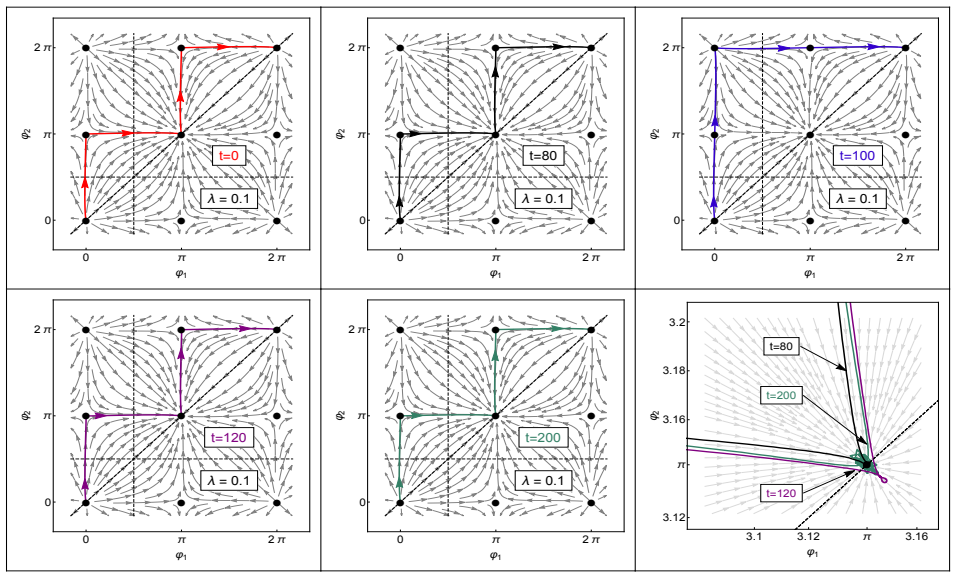
The load-bearing object is the BPS sector defined by the prepotential $U=-4(\cos\phi_1+\epsilon\cos\phi_2)$ together with the modified gradient flow $\nabla_{\gamma}U=\frac{4}{4-\lambda^2}(2\partial_{\phi_1}U+\lambda\partial_{\phi_2}U,\lambda\partial_{\phi_1}U+2\partial_{\phi_2}U)$. The first-order BPS equations are $\partial_x\phi_1=\frac{4}{4-\lambda^2}(4\sin\phi_1+2\lambda\epsilon\sin\phi_2)$ and $\partial_x\phi_2=\frac{4}{4-\lambda^2}(2\lambda\sin\phi_1+4\epsilon\sin\phi_2)$. Because two first-order equations in one dimension leave two constants free, the one-soliton solution carries two zero modes: a global translation and a relative shift of the two fields' soliton positions. It is the relative mode that numerical noise excites, and this is the mechanism that converts an ostensibly static solution into a slow drift. The single-field reduction $\phi_2=\phi_1+\pi$ yields the energy formula $E(\lambda)=8\sqrt{(2-\lambda)/(2+\lambda)}$ used to explain radiation from bound states.
What would settle it
Run the same static BPS initial data at successively smaller lattice spacings (or with successively smaller time steps) and measure the drift speed of the soliton positions; if the extrapolated speed does not tend to zero with the numerical error, the drift is a discretization artefact rather than zero-mode excitation. Alternatively, compute the projection of the initial numerical error onto the relative zero mode and check that the observed drift velocity agrees with it.
Extended reading notes
Core claim
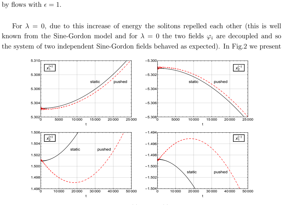
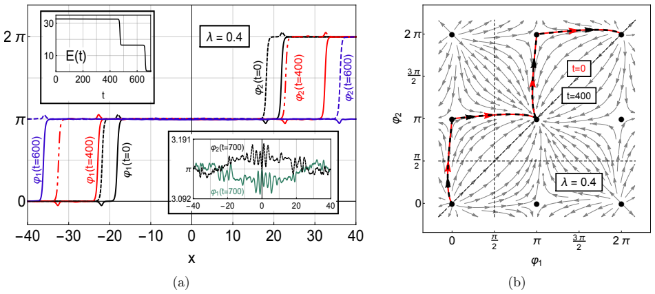
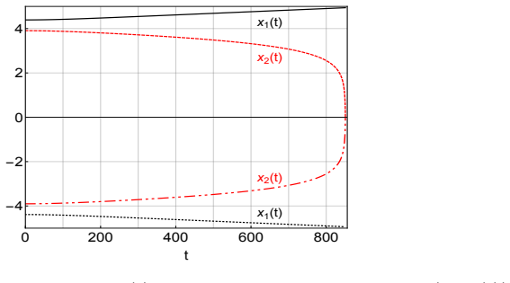
The paper's central discovery, stated in its own terms, is that a BPS solution of a system with two scalar fields and $|\lambda|<2$ has two zero modes, not one: because the BPS equations are first order, the solution depends on two constants, which show up as an overall translation and as a relative motion of the solitons of the two fields. When the equations are evolved numerically, unavoidable round-off error excites the relative zero mode, while momentum conservation kills the translational one. As a result, the 'static' BPS solution evolves very slowly — the paper reports position changes of order $0.05$ to $0.5$ over runs of $10^3$ to $10^4$ time units — with repulsion for kink-antikink systems at $\lambda>0$, attraction at $\lambda<0$, and the opposite signs for two-kink systems, at a rate that grows with $|\lambda|$. The paper also shows that a locked bound state of the two fields can be reinterpreted as a single Sine-Gordon soliton with energy $E(\lambda)=8\sqrt{(2-\lambda)/(2+\lambda)}$, which explains why such bound states radiate their excess energy.
Load-bearing premise
The whole explanation rests on the assumption that the slow motions are caused by numerical noise exciting the relative zero mode, rather than by the discretization scheme or by radiation generated when the initial data are sewn together; the paper reports only global energy conservation to $10^{-5}\%$, not a direct measurement of the numerical error in the modes.
Editorial extensions
If this is right
- Long-time numerical evolutions of multi-field BPS systems cannot be assumed to remain static; the observed slow motions can be numerical artefacts caused by excitation of the relative zero mode.
- For kink-antikink systems, $\lambda>0$ gives a slow repulsion and $\lambda<0$ a slow attraction; for two-kink systems the signs are reversed, and the drift speed increases with $|\lambda|$.
- Studies of multi-soliton interactions at large separation, where the real forces are exponentially small, will be contaminated by this zero-mode drift.
- A locked two-field bound state can be described as one Sine-Gordon soliton with excess energy $E(\lambda)=8\sqrt{(2-\lambda)/(2+\lambda)}$, which explains the late-time radiation and breather emission seen in the simulations.
- The authors expect the same zero-mode artefact in other multi-field BPS solitonic systems, making the warning generic rather than specific to this model.
Reading between the lines
- A convergence study across lattice spacings or time steps would test the mechanism: if the drift is numerical noise exciting a zero mode, its speed should shrink with the numerical error, something the paper does not report.
- One could compute the projection of the numerical error of the initial fields onto the relative zero mode and compare it with the measured drift velocity; if they do not match, the drift has a different source.
- The sign flip between kink-kink and kink-antikink systems might follow from a collective-coordinate effective potential built on the two zero modes; the paper leaves this derivation open.
- If the mechanism is generic, the same slow drift should be observable in other multi-field BPS models, such as coupled $\phi^4$ or baby-Skyrme-type systems, providing a cheap numerical test of the claim.
Signed reviews
Editorial analysis
A structured set of objections, weighed in public.
Referee Report
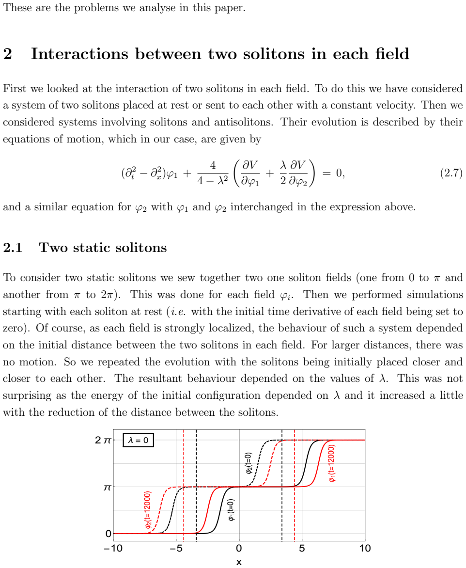
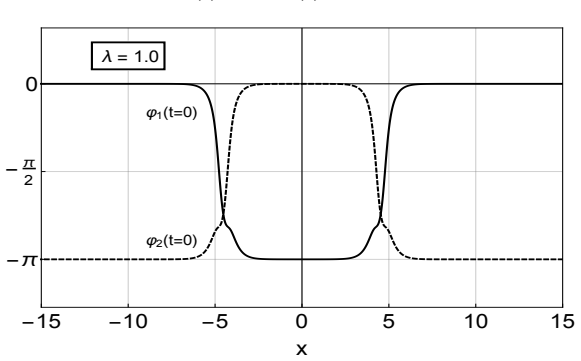
Summary. The paper studies a (1+1)-dimensional model of two coupled sine-Gordon-like scalar fields with a BPS sector, continuing earlier work on the same system. Using numerically determined one-soliton BPS solutions as building blocks, the authors construct two-soliton and kink-antikink initial configurations, evolve them in the Lorentz-covariant field equations, and catalogue their interactions as a function of the coupling λ. They report that two-kink systems repel for small λ but form bound states and emit breathers for larger λ, while kink-antikink systems show sign-dependent attraction/repulsion and oscillon formation. The central new claim, developed in Section 5, is that ostensibly static BPS solutions of the multi-field model slowly drift because tiny numerical errors excite one of the system's zero modes; the direction of the drift is reported to depend on the sign of λ and on the kink/antikink sector. The paper is almost entirely numerical, with no derivation of the drift rate, no convergence study, and no specification of the numerical scheme.
Significance. If the central claim is correct, the paper identifies a practically important phenomenon: long-time numerical simulations of multi-field BPS solitons can exhibit slow, spurious motion along zero-mode directions, which could contaminate studies of soliton interactions. The authors deserve credit for running very long simulations, for reporting energy conservation at the 10^-5% level in several runs, and for clearly separating kink-kink from kink-antikink sectors. The observation that the sign of the drift depends systematically on λ and on the sector is an interesting empirical pattern. However, the paper provides no direct evidence that numerical error projects onto the claimed zero mode, and the authors themselves state at the end of Section 5.4 that they have not explained the sign dependence. Because the entire conclusion rests on the interpretation of numerical observations, the absence of convergence tests, mode-amplitude diagnostics, and a description of the discretization is a serious gap. The result is potentially useful as a cautionary note to the soliton community, but it is not yet established.
major comments (3)
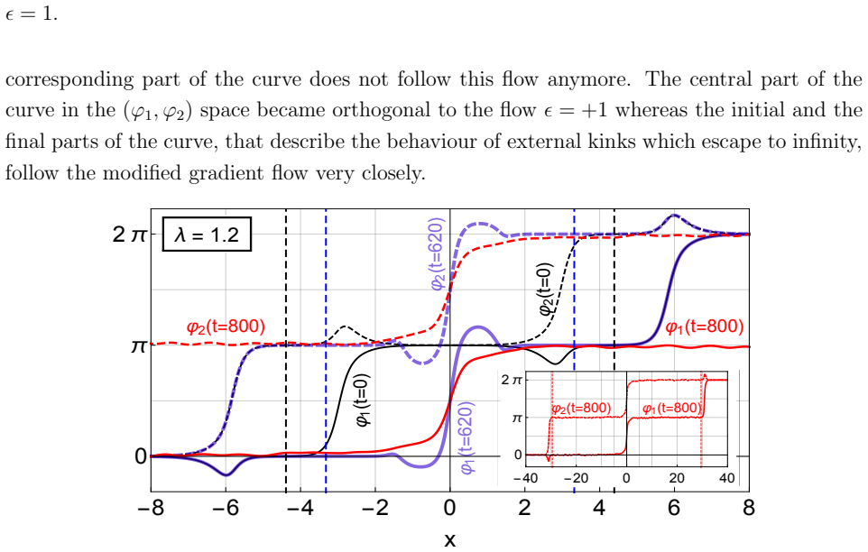
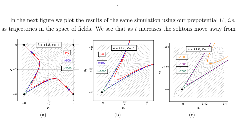
- [§5.3] The central claim that the observed slow drift is caused by excitation of the second zero mode by numerical errors is not supported by any direct measurement. No projection of the initial numerical error, or of the evolving field, onto the two zero modes is reported; no convergence study in dx or dt is given; and no single- versus double-precision comparison is made. Energy conservation to 10^-5% (Figs. 26, 37, 38) cannot constrain motion along a zero mode, because the energy is flat along that direction by definition. In addition, the numerical scheme (discretization, time integrator, grid spacing, time step, boundary treatment) is not described anywhere in the paper, so the reported drifts cannot be checked or reproduced. A refinement study and a mode-projection diagnostic are needed to distinguish genuine zero-mode excitation from a discretization artifact.
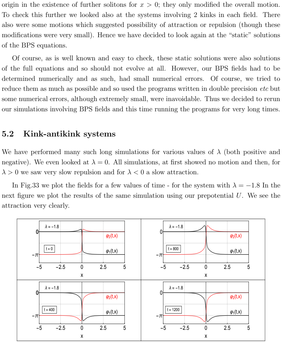
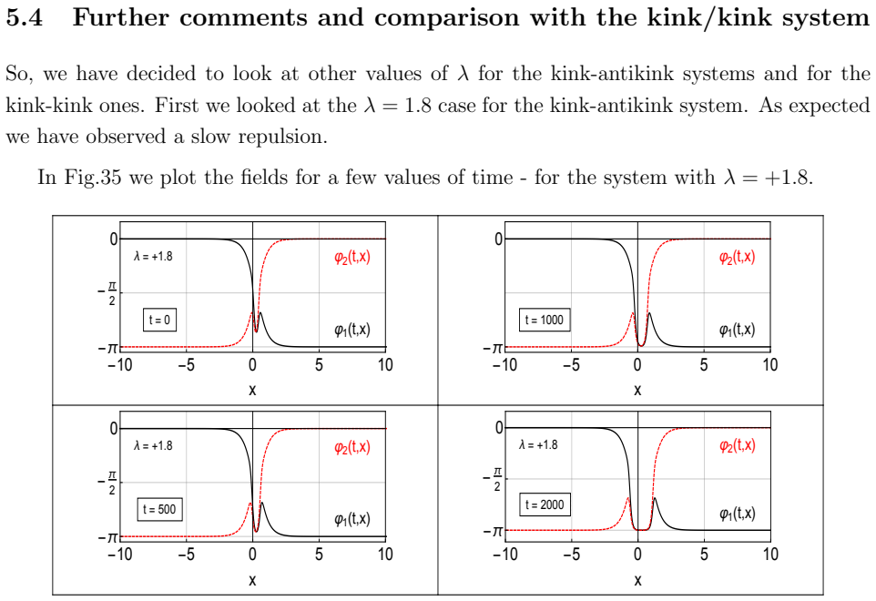
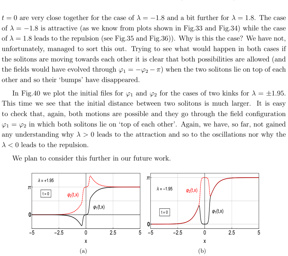
- [§5.4] The systematic sign dependence reported in Figs. 33–38 (attraction for λ<0 in the kink-antikink sector and for λ>0 in the kink-kink sector, with repulsion in the opposite cases) is difficult to attribute to 'small unavoidable numerical errors,' which one would expect to be essentially random. Deterministic discretization error could produce exactly such systematic behavior, which would make the phenomenon an artifact of the numerical scheme rather than generic zero-mode excitation. The authors explicitly concede at the end of Section 5.4 that they have not understood why the sign of λ selects attraction or repulsion; this gap is load-bearing because a zero-mode mechanism should predict the drift direction from the structure of the perturbation. At minimum, the sign of the zero-mode component of the numerical error should be measured and shown to correlate with the observed drift direction.
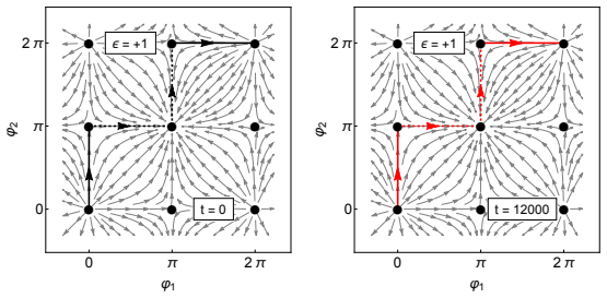
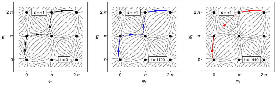
- [§2.1 and §5.2] The paper does not clearly distinguish initial conditions that are exact multi-soliton BPS solutions from configurations obtained by sewing together one-soliton BPS fields at finite separation. Section 2.1 explicitly says that two-soliton initial data are constructed by sewing one-soliton fields, and such sewn configurations are not static solutions of the full equations: they contain radiation from the seam and from the finite-distance interaction. The slow motions observed in Sections 2–4 therefore cannot be used as evidence for the zero-mode mechanism without an estimate of the size of the sewn-data error. Section 5.2 states that 'BPS fields' were determined numerically, but no procedure is given for how the numerical BPS solutions were obtained, how their errors were estimated, or how the initial data were prepared for the long-time runs; this matters because the central claim is that tiny initial errors, not physical forces, drive the drift.
minor comments (5)
- [§2.1.1, Eq. (2.8)] The BPS bound for the energy in Eq. (2.8) is E(λ) = 16√((2−λ)/(2+λ)), not 8√((2−λ)/(2+λ)); at λ=0 this gives 16, matching the two locked kinks, whereas the stated value 8 is the single-field result. The comparison with 'E(λ=1.0)≈4.618' is therefore off by a factor of 2 and should be rechecked.
- [Abstract and §5.3] There are several typos in the abstract and in Section 5.3: 'exitations', 'unevoidable', 'more that one zero mode', and 'inavoidable' should be corrected; similar typos appear throughout the text (e.g., 'fololows', 'looses', 'controlls', 'useed').
- [§4.1 and §5.2] The energy conservation claims are stated inconsistently: the abstract says '10^-5%' while Section 4.1 reports 'up to 10^-7' for one simulation, and some energy plots appear to show box-energy rather than total energy. The diagnostic used for each stated conservation level should be defined precisely.
- [§5.3] The statement that for λ=0 the decoupled system 'sends out only radiation' is supported by a citation to a discrete sine-Gordon paper, but the relevance of that result to the present continuum setup is not explained. Since the λ=0 case is used as the baseline for the zero-mode argument, a brief derivation or explicit numerical demonstration would be helpful.
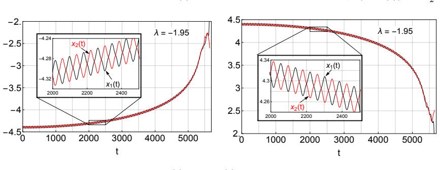
- [References and figures] Reference [6] has an incomplete arXiv identifier ('arXiv: 1206.447' is missing digits), and reference [8] is missing a period. In Fig. 24 the y-axis label '4.' should read '4.0', and in the caption of Fig. 28 'λ−1.95' should read 'λ=−1.95'.
Circularity Check
No significant circularity: the central claims are numerical observations, not derivations reducible to their inputs.
full rationale
The paper's main claims are empirical: multi-kink and multi-antikink configurations evolve in certain ways, and long-time runs of ostensibly static BPS solutions show very small drifts attributed to excitation of zero modes by numerical errors. These are observations supported by simulations, not quantities fitted to make a predicted result emerge. The BPS model and equations (1.1)-(1.5) are adopted from the authors' earlier paper [1], but that is background definition, not a circular derivation; the paper's new findings about slow attraction/repulsion as a function of the sign of lambda, zero-mode drift, and energy conservation are not obtained by invoking the same conclusion under a new name. The reduced energy expression (2.8) is obtained by substituting the bound-state relation phi2 = phi1 + pi into the theory, and it is used to explain radiation of excess energy rather than to force a target outcome. Section 5.3's zero-mode argument counts integration constants of the first-order BPS equations and invokes momentum conservation; it does not import a uniqueness theorem from the authors' prior work. Whether the zero-mode attribution is fully established is a numerical-evidence question, not a circularity question: the paper does not report a convergence study or a projection of numerical error onto the zero mode, but absence of such evidence is a robustness concern, not a reduction of the conclusion to its input. No fitted parameter is renamed as a prediction, and no self-citation carries the load of the central claim. The paper is therefore self-contained with respect to circularity.
Assumptions & free parameters
free parameters (3)
- lambda (coupling strength) =
scanned values include +/-0.1, +/-0.4, +/-0.6, +/-0.8, +/-1.0, +/-1.2, +/-1.5, +/-1.8, +/-1.95
- initial soliton separations =
not tabulated per run
- numerical grid parameters =
not reported (dx, dt, stencil)
assumptions (4)
- domain assumption The two-field model has BPS solutions that are well-localized single-kink profiles.
- domain assumption Sewing together one-soliton profiles yields valid approximate multi-soliton configurations.
- ad hoc to paper Numerical round-off errors behave as small perturbations that excite only the system's zero modes.
- domain assumption Energy conservation to about 10^-5 percent is sufficient to trust very slow motions.
Cite this review
Pith. "Pith review of Further comments on BPS systems." pith.science (2026). https://pith.science/paper/HVQ3XMWU
@misc{pith2026190802100,
  author       = {Pith},
  title        = {Pith review of: Further comments on BPS systems},
  year         = {2026},
  howpublished = {\url{https://pith.science/paper/HVQ3XMWU}},
  note         = {Machine review of arXiv:1908.02100}
}
abstract
We look at BPS systems involving two interacting Sine-Gordon like fields both when one of them has a kink solution and the second one either a kink or an antikink solution. The interaction between the two fields is controlled by a parameter $\lambda$ which has to satisfy $| \lambda|< 2$. We then take these solitonic static solutions (with solitons well localised) and construct from them systems involving two solitons in each field (kinks and antikinks) and then use them as initial conditions for their evolution in Lorentz covariant versions of such models. This way we study their interactions and compare them with similar interactions involving only one Sine-Gordon field. In particular, we look at the behaviour of two static kinks in each field (which for one field repel each other) and of a system involving kinks and anti-kinks (which for one field attract each other) and look how their behaviour depends on the strength of the interaction $\lambda$ between the two fields. Our simulations have led us to look again at the static BPS solutions of systems involving more fields. We have found that such ostensibly 'static' BPS solutions can exhibit small motions due to the excitation of their zero modes. These excitations arise from small unavoidable numerical errors (the overall translation is cancelled by the conservation of momentum) but as systems of two or more fields have more that one zero mode such motions can be generated and are extremely small. The energy of our systems has been conserved to within $10^{-5}\%$.
Figures

Figures from the paper (37 more)










Forward citations
Cited by 1 Pith paper
-
Kinks in generalized scalar field models and their scattering properties
Absolute-value couplings in scalar field superpotentials produce kinks that compactify with n, and collisions of these kinks lose two-bounce windows as the number of vibrational bound states grows.
Reference graph
Works this paper leans on
-
[1]
L. A. Ferreira, P. Klimas, A. Wereszczynski and W. J. Zakrzewski, “Some Comments on BPS systems,” (arXiv:1803.08985)
-
[2]
Solitons in systems of coupled scalar fields
D. Bazeia, M.J. dos Santos , R.F. Ribeiro, “Solitons in systems of coupled scalar fields”, Phys. Lett. A208, 84 (1995)
work page 1995
-
[3]
Some aspects of self-duality and generalised BPS theories
C. Adam, L. A. Ferreira, E. da Hora, A. Wereszczynski and W. J. Zakrzewski, “Some aspects of self-duality and generalised BPS theories,” JHEP1308, 062 (2013) [arXiv:1305.7239 [hep-th]]
work page Pith review arXiv 2013
-
[4]
The First-Order Euler-Lagrange equations and some of their uses
C. Adam and F. Santamaria, “The First-Order Euler-Lagrange equations and some of their uses,” [arXiv:1609.02154 [hep-th] 2016
work page Pith review arXiv 2016
-
[5]
The concept of quasi-integrability: a concrete example
L.A. Ferreira and W.J. Zakrzewski, “The concept of quasi-integrability: a concrete example. ”JHEP 05 130 (2011); arXiv:1011.2176 (hep-th) (2010)
work page Pith review arXiv 2011
-
[6]
Resonance structure in couple two-componentλφ4 model
A. Halavanau, T. Romanczukiewicz and Ya. Shnir, “Resonance structure in couple two-componentλφ4 model”; arXiv: 1206.447 (hep-th) (2012)
work page 2012
-
[7]
Self-dual sectors for scalar field theories in (1 + 1) dimensions
L.A. Ferreira, P. Klimas and W.J. Zakrzewski, “Self-dual sectors for scalar field theory in (1+1) dimensions”; arXiv: 1808.10052 (hep-th) (2018)
work page Pith review arXiv 2018
-
[8]
see e.g. M.J. Ablowitz and P.A. Clarkson, “Solitons, Nonlinear Evolution Equations and Inverse Scattering’; London Mathematical Lecture Note Series, Vol 149, CUP, Cam- bridge (1991)
work page 1991
Show all 10 references
-
[9]
An effective Lagrangian for Solitons
N.S. Manton, “An effective Lagrangian for Solitons”, Nuclear Physics B 150, 397-412 (1979)
1979
-
[10]
Spontaneous emission of radiation from a discrete sine-Gordon kink
R. Boesch, C.R. Willis and M. El-Batanouny, “Spontaneous emission of radiation from a discrete sine-Gordon kink”, Phys. Rev. B40, 2284 (1989). 31
1989
Reviewed August 14, 2026 · model on record in the stance chip above.
Discussion (0). Continue with ORCID to comment.