REVIEW 3 major objections 6 minor 1 cited by
Knapsack Problem variants of QAOA for battery revenue optimisation
T0 review · 3 major / 6 minor · reviewed 2026-08-14 · deepseek-v4-flash
Pith's one-line read This paper tries to establish that a relaxed, non-Ising QAOA encoding of the knapsack constraint reaches about 0.95 of the optimal battery revenue with shallow depth (p ≤ 10) and shows exponential improvement in depth, whereas the Ising…
desk verdict The non-Ising QAOA with a reversible-arithmetic linear penalty is a real idea, but the paper's headline 0.95 claim is measured against the penalized objective, not the constrained knapsack optimum, so the performance claim needs re-scoring before it can be trusted. read the letter →
The pith
A machine-rendered reading of the paper's core claim, the machinery that carries it, and where it could break.
The reading
What carries the argument
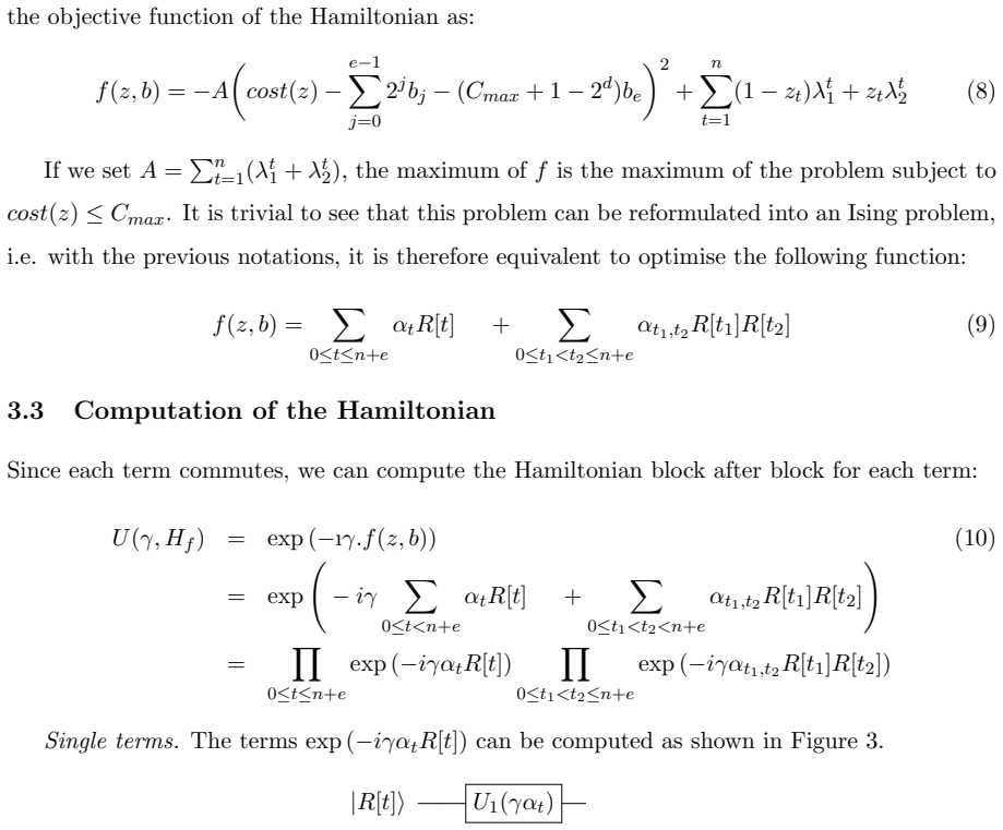
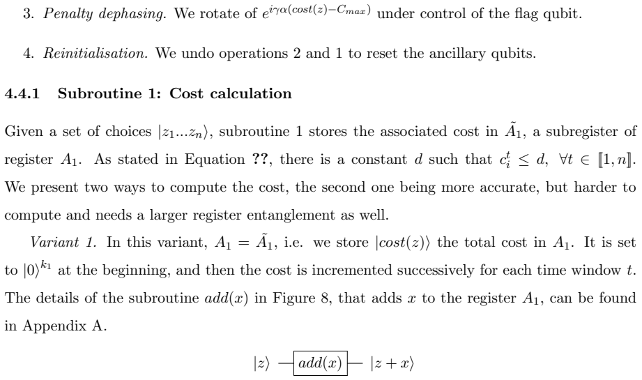
The key object is the non-Ising target Hamiltonian whose phase operator U(C, γ) = $e^{{-iγ f(z)}}$ is built from four subroutines: cost calculation, constraint testing with a flag qubit, penalty dephasing, and reinitialisation by uncomputation. The linear penalty is enforced by rotating the flag-controlled phase by $e^{{iγα(cost(z)−Cmax)}}$, which makes the constraint violation enter the objective linearly rather than quadratically. This construction is what allows the relaxed approach to avoid the heavy quadratic penalty that stalls the Ising formulation.
What would settle it
Run the relaxed QAOA on the same random instance family with n = 10 and p = 12 while re-optimising the angles β, γ instead of using the fixed schedule; if the average approximation ratio falls below 0.9, the claim that shallow fixed-schedule depth suffices would be contradicted.
Extended reading notes
Core claim
The central claim is that QAOA can approximate the optimal battery schedule by encoding the knapsack constraint as a linear penalty in the objective function rather than as a quadratic Ising penalty. The relaxed objective is f(z) = return(z) + penalty(z), where penalty(z) is zero when the cycle budget is respected and −α(cost(z) − Cmax) otherwise. The circuit uses O(n log n) qubits and has depth O(p(log n)^3), with the phase separation implemented through addition circuits, a constraint-testing flag, and controlled dephasing. Simulations on a qubit-level simulator report approximation ratios around 0.95 for p ≤ 10 and an exponential improvement in p, while the Ising constrained variant plateaus near 0.75 for p ≤ 50.
Load-bearing premise
The reported 0.95 approximation assumes that the fixed linear annealing schedule (β_k = 1 − k/p, γ_k = k/p) and the penalty coefficient α = 1 work on the small random instances tested; if these choices do not generalise, the exponential improvement and near-optimal ratios do not transfer.
Editorial extensions
If this is right
- Battery revenue schedules can be approximated with shallow QAOA circuits using the relaxed non-Ising encoding, provided the fixed angle schedule is kept.
- The quadratic-penalty Ising route is not effective for this problem at shallow or intermediate depth, so further work on constrained QAOA should consider linear penalty encodings.
- The circuit's depth O(p(log n)^3) and qubit count O(n log n) make the approach implementable for small problem sizes on near-term devices.
- Linear constraints of the form sum w_t z_t ≤ Cmax can be handled in QAOA by the flag-controlled linear penalty technique, not only for knapsack but for a wider class of constrained binary optimisation problems.
Reading between the lines
- If the observed exponential improvement in depth persists at larger n, QAOA with a linear penalty could become a competitive heuristic for small knapsack instances, though this remains to be tested beyond n ≤ 7.
- The fixed linear annealing schedule (β_k = 1 − k/p, γ_k = k/p) is likely not optimal; re-optimising the angles could push approximation ratios higher or reveal a different scaling with p.
- The penalty coefficient α = 1 was chosen arbitrarily; varying α could trade off constraint satisfaction against revenue and might be necessary for problems with different return/cost scales.
- The same relaxation strategy could apply to other weakly NP-hard problems with a single linear constraint, such as subset sum, where Ising penalties are known to create heavy objective weights.
Signed reviews
Editorial analysis
A structured set of objections, weighed in public.
Referee Report
Summary. The paper implements two QAOA variants for a battery revenue optimization problem modeled as a knapsack problem. The first variant enforces the capacity constraint through a quadratic penalty and an Ising reformulation, but simulations show non-convergent behavior for intermediate circuit depths. The second, 'relaxed' variant uses a non-Ising objective with a linear penalty, implemented with arithmetic and flag-qubit subroutines, and is claimed to run in O(p(log_2 n)^3) time with O(n log n) qubits. The main reported result is a roughly 0.95 approximation ratio of the optimal penalized objective at shallow depth (p <= 10), with an exponential improvement in the ratio as p increases. The paper concludes that the linear-penalty QAOA is a promising way to handle constrained problems with shallow circuits.
Significance. If the central claim is established after correcting the evaluation baseline, the paper would be a useful proof-of-concept for applying QAOA to constrained, non-Ising optimization problems. The proposed circuit construction for computing a linear penalty is novel and nontrivial, and the explicit complexity estimates (polylogarithmic depth in n, O(n log n) qubits) are valuable. The paper also provides concrete simulation tables over random instances and is honest about the arbitrary choice of alpha. However, the current evidence does not yet support the abstract's near-optimality claim because the reported ratios are measured against the penalized objective rather than the feasible knapsack optimum, and the statistical support for the exponential-improvement claim is thin.
major comments (3)
- [Section 5.1 and 5.3.2, Eq. (12)] The reported approximation ratios for the with-penalty experiments are measured against the penalized objective f(z) = return(z) + penalty(z), not against the original feasible knapsack optimum. Section 5.1 defines the ratio as 'the value of the output of the algorithm over the optimal value for the chosen target function,' and in Section 5.3.2 the target function includes the linear penalty with alpha = 1. A finite linear penalty does not enforce the capacity constraint: with Cmax = n, c_t^1 = 2, lambda_t^1 = 5, lambda_t^2 = 0, the all-M1 schedule has return 5n, cost 2n, and penalized value 4n, while the best feasible value is about 2.5n. Thus ratios near 0.95 against the penalized optimum do not imply 0.95 of the feasible optimum. The paper reports no constraint-violation rate and no comparison against the optimal feasible schedule. Re-scoring the simulated outputs against the feasible optimum is required before the abstract's claim can be accepted; the 'without penalty' experiments do not provide such a benchmark because they solve an unconstrained selection problem.
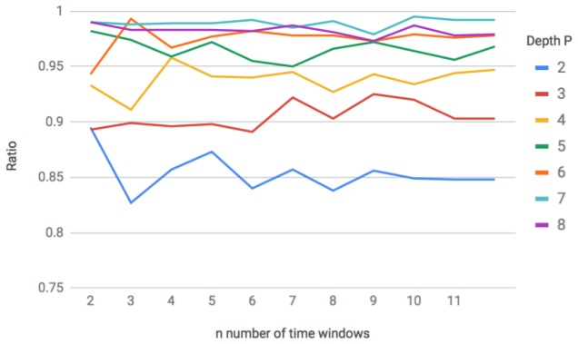
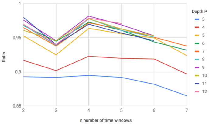
- [Section 5.3.2, Table 3 and Figures 17-18] The 'exponential improvement' claim is not statistically supported. The tables report only mean ratios over 1000 random instances, with no standard deviations, confidence intervals, or significance tests. The with-penalty results stop at n = 7 and contain missing entries for n = 6 at p >= 9 and for n = 7 at p >= 7, while the text refers to behavior for n = 8 without data. With one mean per condition, the reader cannot assess whether the apparent improvement with p is real or within sampling noise, nor can the functional form of the claimed exponential improvement be checked. The authors should report distributions or error bars and specify the fitted curve used to infer exponential scaling.
- [Section 2.2 and Section 5.3.2] The fixed linear annealing schedule beta_k = 1 - k/p, gamma_k = k/p and the penalty coefficient alpha = 1 are untested hyperparameters. The paper itself states that alpha = 1 is 'arbitrary.' Since the central near-optimality result depends on these choices, the claim should either be tested over a range of alpha values and at least one alternative angle schedule, or explicitly stated as conditional on these specific choices. Without such testing, the reported approximation ratios could be specific to this parameter setting rather than a property of the algorithm.
minor comments (6)
- [Section 4.4] The text says 'We present below two implementations to compute e^{-i*gamma*return(z)}' but the surrounding discussion is about the penalty part; this appears to be a typo for the penalty Hamiltonian.
- [Section 4.4.1] In the introduction to Subroutine 1, 'As stated in Equation ??' has an unresolved equation reference; the bound d = max c_t^i should be stated explicitly at first use.
- [Section 5.3.2] The text says 'It seems to sink for n = 8' but Table 3 contains no n = 8 row; either add the data or remove the speculation.
- [Table 3] Several entries read 'NO DAT'; these should be replaced with actual values or the reasons for their absence should be explained in the caption.
- [Appendix B] The complexity derivation is a sketch: the number of steps and the ancillary-qubit count are described in words, and the phrase 'The subroutine 2 takes therefore a shortest time' should read 'a shorter time.' A more formal accounting of circuit depth and qubit reuse would make the O(p(log n)^3) and O(n log n) claims easier to verify.
- [Figures 16 and 18] The figures plot 'ratio versus P' but do not state what quantity is used to infer an exponential improvement; the authors should define the plotted data and describe any fitted curve in the captions.
Circularity Check
No significant circularity: the reported ratios are measured against independently computed optima, and the QAOA angles and penalty coefficient are fixed modeling choices rather than fitted inputs.
full rationale
The paper's central empirical claim is that the relaxed QAOA reaches approximation ratios near 0.95 with shallow depth. The derivation chain does not reduce to its inputs by construction. The angles are set to the fixed linear annealing schedule beta_k = 1 - k/p and gamma_k = k/p (Section 2.2), and the penalty coefficient is explicitly stated as arbitrary with alpha = 1 (Section 5.3.2); neither is fitted to the simulation outcomes. The approximation ratio is defined in Section 5.1 as 'the value of the output of the algorithm over the optimal value for the chosen target function,' which is computed for each random instance. Thus the ratio is an external benchmark against exact optima of the objective actually used by the circuit, not a restatement of a fitted parameter. The concern that the penalized target function may differ from the feasible knapsack optimum is a benchmark-validity and correctness question, not a circularity: the paper does not define the optimum in terms of the algorithm's output, and no equation in the paper equates the claimed result with an input assumption. There are no load-bearing self-citations, no imported uniqueness theorems, and no ansatz presented as derived when it was in fact postulated. The paper is self-contained as a simulation study, and any weakness in the central claim is an empirical or modeling limitation rather than a circular derivation.
Assumptions & free parameters
free parameters (2)
- alpha (penalty coefficient) =
1
- QAOA angle schedule =
beta_k = 1 - k/p, gamma_k = k/p
assumptions (4)
- standard math The adiabatic theorem guarantees QAOA converges to the optimum as p goes to infinity.
- domain assumption Battery state resets every day, so time windows are independent and intraday charging dynamics are ignored.
- domain assumption Battery degradation is characterized only by a maximum cycle count and known daily costs c_t^1, c_t^2.
- domain assumption d = max_t c_t^i is O(1).
Cite this review
Pith. "Pith review of Knapsack Problem variants of QAOA for battery revenue optimisation." pith.science (2026). https://pith.science/paper/CMI42ATK
@misc{pith2026190802210,
  author       = {Pith},
  title        = {Pith review of: Knapsack Problem variants of QAOA for battery revenue optimisation},
  year         = {2026},
  howpublished = {\url{https://pith.science/paper/CMI42ATK}},
  note         = {Machine review of arXiv:1908.02210}
}
abstract
We implement two Quantum Approximate Optimisation Algorithm (QAOA) variants for a battery revenue optimisation problem, equivalent to the weakly NP-hard Knapsack Problem. Both approaches investigate how to tackle constrained problems with QAOA. A first 'constrained' approach introduces a quadratic penalty to enforce the constraint to be respected strictly and reformulates the problem into an Ising Problem. However, simulations on IBM's simulator highlight non-convergent results for intermediate depth ($ p\leq 50$). A second 'relaxed' approach applies the QAOA with a non-Ising target function to compute a linear penalty, running in time $O(p(\log_2 n)^3)$ and needing $O(n \log n)$ qubits. Simulations reveal an exponential improvement over the number of depth levels and obtain approximations about $0.95$ of the optimum with shallow depth ($p \leq 10$).
Figures


Figures from the paper (18 more)






Forward citations
Cited by 1 Pith paper
-
Quadratic versus Polynomial Unconstrained Binary Models for Quantum Optimization illustrated on Railway Timetabling
On three tiny railway-timetabling instances, QAOA with a polynomial (PUBO) encoding returned optimal feasible solutions in 55-71% of runs versus 4-8% for a quadratic (QUBO) encoding.
Reference graph
Works this paper leans on
-
[1]
Qiskit: An Open-source Framework for Quantum Computing (v 0.11.1)
Gadi Aleksandrowicz et al. Qiskit: An Open-source Framework for Quantum Computing (v 0.11.1) . 2019. doi: 10.5281/zenodo.2562110 . url: https://github.com/Qiskit/ qiskit
-
[2]
An Elementary Proof of the Quantum Adiabatic Theorem
Oded Regev Andris Ambainis. “An Elementary Proof of the Quantum Adiabatic Theorem” (2018). url: http://arxiv.org/abs/quant-ph/0411152
arXiv 2018
-
[3]
Adiabatic quantum computing solution of the knapsack problem
Mark W. Coffey. “Adiabatic quantum computing solution of the knapsack problem” (2017), pp. 1–22. arXiv: 1701.05584. url: http://arxiv.org/abs/1701.05584
work page Pith review arXiv 2017
-
[4]
Quantum Algorithm Implementations for Beginners
Patrick J. Coles et al. “Quantum Algorithm Implementations for Beginners” (2018). arXiv: 1804.03719. url: http://arxiv.org/abs/1804.03719
arXiv 2018
-
[5]
Performance of the Quantum Approximate Optimization Algorithm on the Maximum Cut Problem
Gavin E Crooks. “Performance of the Quantum Approximate Optimization Algorithm on the Maximum Cut Problem” (2018), pp. 15–17
work page 2018
-
[6]
A Quantum Approximate Opti- mization Algorithm
Edward Farhi, Jeffrey Goldstone, and Sam Gutmann. “A Quantum Approximate Opti- mization Algorithm” (2014). arXiv: 1411.4028. url: http://arxiv.org/abs/1411.4028
arXiv 2014
-
[7]
A quantum adiabatic evolution algorithm applied to random instances of an NP-complete problem
Edward Farhi et al. “A quantum adiabatic evolution algorithm applied to random instances of an NP-complete problem”. Science 292.5516 (2001), pp. 472–475
work page 2001
-
[8]
Lecture on Approximations Algorithms
Anupam Gupta. Lecture on Approximations Algorithms. Topic: Dynamic Programming
Show all 18 references
-
[9]
Factoring using 2n+2 qubits with Toffoli based modular multiplication
Thomas H¨ aner, Martin Roetteler, and Krysta M. Svore. “Factoring using 2n+2 qubits with Toffoli based modular multiplication” (2016). arXiv: 1611 . 07995. url: http : / / arxiv.org/abs/1611.07995
2016 arXiv
-
[10]
Optimizing electric vehicle charging with energy storage in the electricity market
Chenrui Jin, Jian Tang, and Prasanta Ghosh. “Optimizing electric vehicle charging with energy storage in the electricity market”. IEEE Transactions on Smart Grid 4.1 (2013), pp. 311–320
2013
-
[11]
Reducibility among combinatorial problems
Richard M Karp. “Reducibility among combinatorial problems”. Complexity of computer computations. Springer, 1972, pp. 85–103
1972
-
[12]
Bidding strategy for microgrid in day-ahead market based on hybrid stochastic/robust optimization
Guodong Liu, Yan Xu, and Kevin Tomsovic. “Bidding strategy for microgrid in day-ahead market based on hybrid stochastic/robust optimization”. IEEE Transactions on Smart Grid 7.1 (2015), pp. 227–237
2015
-
[13]
Multi-objective optimization of energy arbitrage in community energy storage systems using different battery technologies
Tom Terlouw et al. “Multi-objective optimization of energy arbitrage in community energy storage systems using different battery technologies”. Applied Energy 239 (2019), pp. 356– 372. 28
2019
-
[14]
Quantum networks for elementary arithmetic operations
Vlatko Vedral, Adriano Barenco, and Artur Ekert. “Quantum networks for elementary arithmetic operations”. Physical Review A - Atomic, Molecular, and Optical Physics 54.1 (1996), pp. 147–153. issn: 10941622. doi: 10.1103/PhysRevA.54.147
1996 doi
-
[15]
Quantum Optimization for Maximum Independent Set Using Rydberg Atom Arrays
Guillaume Verdon, Michael Broughton, and Jacob Biamonte. “Quantum Optimization for Maximum Independent Set Using Rydberg Atom Arrays” (2017), pp. 1–8
2017
-
[16]
An Introduction to Quantum Optimization Approx- imation Algorithm
Qingfeng Wang and Tauqir Abdullah. An Introduction to Quantum Optimization Approx- imation Algorithm. Tech. rep. 2018
2018
-
[17]
Quantum Approximate Optimization Algorithm: Performance, Mecha- nism, and Implementation on Near-Term Devices
Leo Zhou et al. “Quantum Approximate Optimization Algorithm: Performance, Mecha- nism, and Implementation on Near-Term Devices” (Dec. 2018). url: http://arxiv.org/ abs/1812.01041. 29
2018 arXiv
-
[2005]
url: http://www.cs.cmu.edu/afs/cs/academic/class/15854-f05/www/
Reviewed August 14, 2026 · model on record in the stance chip above.
Discussion (0). Continue with ORCID to comment.