REVIEW 4 major objections 5 minor 1 cited by
Continuous Graph Flow
T0 review · 4 major / 5 minor · reviewed 2026-08-14 · deepseek-v4-flash
Pith's one-line read Continuous Graph Flow turns graph message passing into an ODE, gains exact likelihoods, and reports the best generative results on three graph tasks.
desk verdict The continuous-time message passing idea is real, but the main empirical evidence is invalid as reported and the rest is mixed. read the letter →
The pith
A machine-rendered reading of the paper's core claim, the machinery that carries it, and where it could break.
The reading
What carries the argument
The central machinery is the continuous message-passing ODE of Eq. (10): each node's instantaneous change is an aggregation \(g\) of shared pairwise message functions \(\hat f_{ij}\) evaluated on the node and its neighbors. Integration from \(t_0\) to \(t_1\) turns a simple base density into the data density, and the continuous change-of-variables formula \(\log p(X(t_1))=\log p(X(t_0))-\int_{t_0}^{t_1}\operatorname{Tr}(\partial F/\partial X(t))\,dt\) supplies exact likelihoods. The trace is made tractable with Hutchinson's estimator, so the Jacobian is unrestricted rather than constrained by coupling layers. A multi-scale variant stacks flow blocks with a factor-out step after each block, following the real NVP design. This machinery is what makes the model reversible, memory-efficient during training, and able to be applied to any graph size.
What would settle it
Re-running any Table 2 or Table 3 configuration with the same preprocessing and likelihood protocol for the baselines as for CGF would settle the comparison; if the reported lead in bits/dimension or per-node NLL collapses, the central claim fails. A second check is to inspect the learned vector field for finite-time blow-up on held-out inputs, since the trace formula in Eq. (13) is exact only for Lipschitz dynamics.
Extended reading notes
Core claim
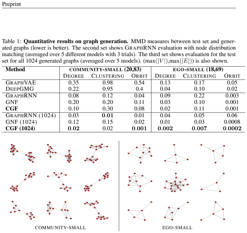
The central claim is that neural message passing over a graph can be posed as continuous-time dynamics and used as a density model. Each node's value evolves under an ODE whose right-hand side aggregates shared pairwise message functions over the node's neighbors, so the same trained functions apply to any graph. Solving this ODE from a simple base distribution to the data distribution is a normalizing flow, making the log-likelihood the base log-likelihood minus the time-integral of the trace of the Jacobian of the combined dynamics; the trace is estimated with Hutchinson's noise vector. The authors report lower MMD under the 1024-graph protocol on the two graph benchmarks, about 2 to 3.5 bits/dimension lower negative log-likelihood on image puzzles, and several units lower per-node negative log-likelihood on scene-graph layouts than the best compared baselines, plus generalization to unseen graph sizes in the puzzle task. They attribute the advantage to free-form Jacobians, which avoid the architectural constraints of coupling-layer flows.
Load-bearing premise
The headline wins presuppose that every model was scored under the same data preprocessing and likelihood protocol, and that the learned continuous-time dynamics are smooth enough for the exact likelihood formula to hold.
Editorial extensions
If this is right
- A single trained CGF can be decoded on graphs of any node count, so graph-size generalization is a property of the dynamics rather than a retraining requirement.
- Exact likelihoods let practitioners compare models directly and do model selection without variational bounds or importance-weighting corrections.
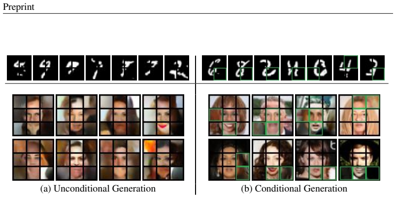
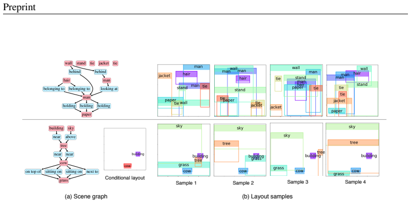
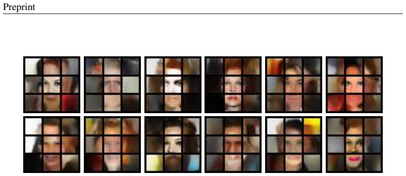
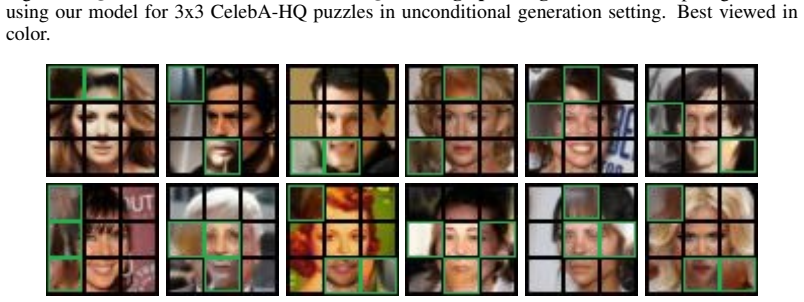
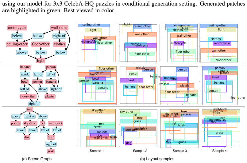
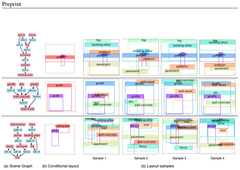
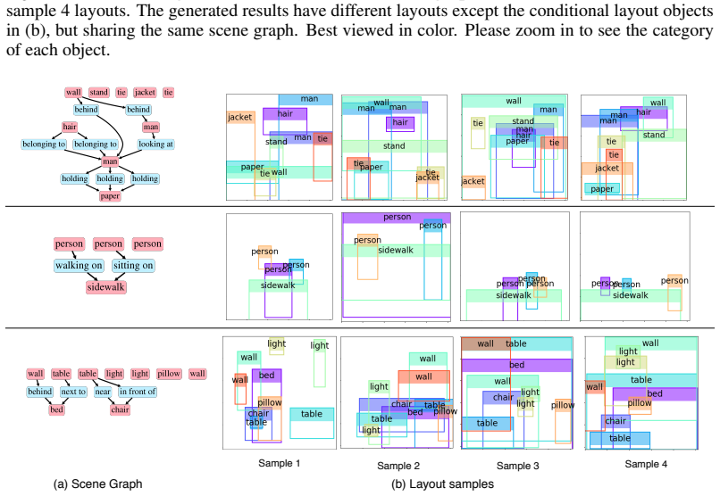
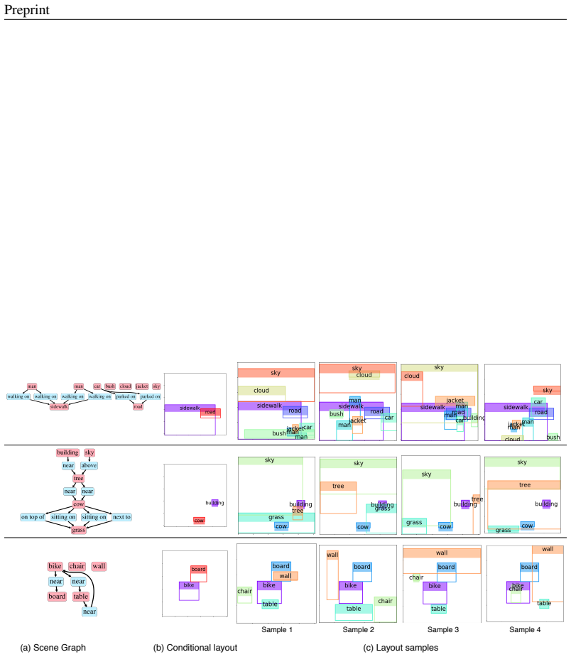
- The same flow supports unconditional sampling from a Gaussian base and conditional generation by fixing a subset of node values and integrating the rest, as shown in the puzzle-completion and conditional-layout experiments.
- On the three reported tasks, CGF's numbers are consistently below the best compared baselines, indicating the improvement is not confined to one data type.
Reading between the lines
- Not tested in the paper: whether one CGF with fixed message functions can generate several graph families at once; the shared-function design suggests it could, but the experiments train separate models per dataset.
- Because the flow is continuous, integrating partway between two graph states may produce meaningful interpolations; the paper does not investigate this, but it is an immediate consequence of the ODE formulation.
- The image-puzzle protocol does not specify dequantization or normalization for continuous pixel data, so exact-likelihood comparisons with baselines may depend on details the paper leaves open.
Signed reviews
Editorial analysis
A structured set of objections, weighed in public.
Referee Report
Summary. The paper introduces Continuous Graph Flow (CGF), a generative model for graph-structured data that generalizes discrete neural message passing to continuous time via an ODE system with shared graph message functions. The log-density of the transformed variables is obtained through the instantaneous change-of-variables formula with Hutchinson trace estimation. The authors evaluate CGF on graph generation, image puzzle generation, and scene graph layout generation, reporting strong quantitative gains over several baselines and claiming exact and efficient likelihood computation as well as generalization to unseen graph sizes.
Significance. If the results are correct, CGF is a conceptually clean extension of continuous normalizing flows to graph-structured data, with the attractive properties of shared and reusable message functions, dimension-agnostic inference, and a tractable density. The mathematical formulation in Eqs. (10)--(13) is a standard and sound application of the continuous change-of-variables formula, and the generalization experiments in Sec. 4.4 are a useful addition that goes beyond mere curve fitting on fixed graph sizes. However, the empirical claims rest on likelihood comparisons whose validity is not currently established, especially for the image-puzzle task, and the paper's own Table 1 does not uniformly support the headline claim of significantly better performance.
major comments (4)
- [Sec. 4.2 and Appendix A.1] The image-puzzle NLL values in Table 2 are not valid data likelihoods as reported. Appendix A.1 states that each puzzle patch is transformed by a convolutional layer into an embedding of size 64 before message passing, and Eq. (13) computes the density on those embeddings. For Eq. (13) to be an exact likelihood of the original patch, the embedding must be invertible and its log-determinant must appear in the change of variables; neither is provided. In addition, MNIST, CIFAR-10, and CelebA pixels are discrete 8-bit values, and Appendix A.1 explicitly applies variational dequantization only for graph generation, not for image puzzles. A continuous density evaluated on non-dequantized discrete data is not a comparable likelihood. The 1--3 bit/dim gaps in Table 2 therefore do not support the claimed superiority over the VAE baselines unless the authors specify an invertible embedding and a dequantization or discretization protocol.
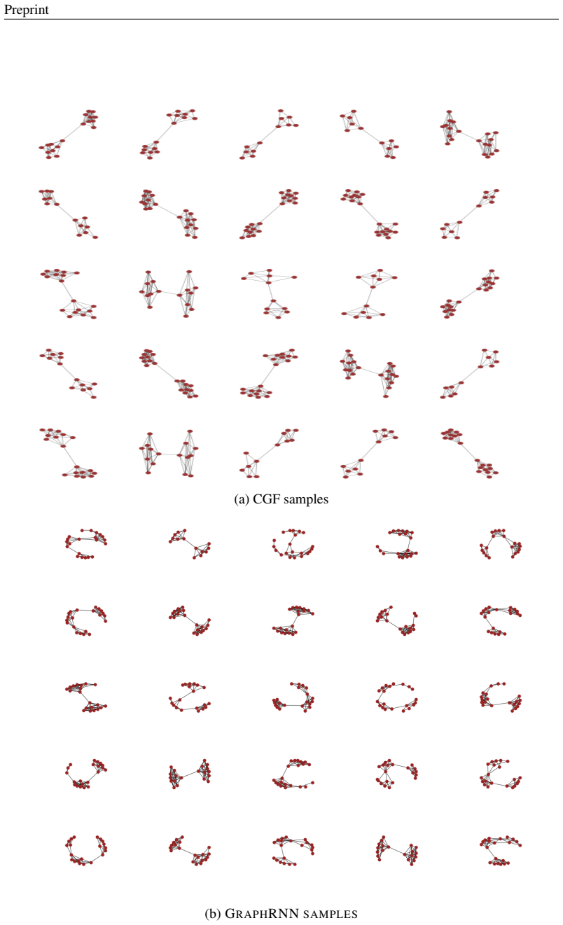
- [Table 1 and Sec. 4.1] The abstract's claim of 'significantly better performance compared to state-of-the-art models' is contradicted by the first evaluation block of Table 1 on COMMUNITY-SMALL, where GraphRNN achieves better MMD than CGF on all three metrics (degree 0.08 vs 0.10, clustering 0.12 vs 0.30, orbit 0.04 vs 0.08). CGF improves on GraphRNN only in the second 1024-sample evaluation block. The authors should clarify which evaluation protocol supports the headline claim, and should report variance or significance estimates rather than selecting the protocol under which the model wins.
- [Abstract and Sec. 3.2, Eq. (14)] The claim of 'exact and efficient computation of the likelihood' is overstated as implemented. Eq. (14) computes the log-likelihood using a Hutchinson trace estimator combined with a numerical ODE solver; the result is an unbiased stochastic estimate with solver tolerance error, not an exact value. The authors should temper the wording or state explicitly that the reported NLL values are stochastic estimates obtained with a fixed tolerance and trace-sample count.
- [Secs. 4.2--4.3 and Tables 2--3] The comparisons with VAE baselines may not be apples-to-apples. For discrete image data, the VAE baselines typically report variational lower bounds on the log-likelihood, while CGF is presented as an exact density; for the layout task, no likelihood protocol (e.g., normalization, output parameterization, or dequantization of any discrete objects) is given for any model. Unless all models were evaluated under the same preprocessing and with the same type of likelihood estimate, the large gaps in Tables 2 and 3 are not interpretable as relative generative quality.
minor comments (5)
- [Sec. 2, Eq. (5)] Eq. (5) is missing the logarithm and the minus sign: the stated dynamics of the log-likelihood should be d log p(z(t))/dt = -Tr(df/dz(t)), not d p(z(t))/dt = Tr(df/dz(t)).
- [Sec. 4.4] The description of the generalization settings contains a clear copy-paste error: the sentence defining 'less to more' is repeated for 'more to less', and the two settings are not actually distinguished.
- [Appendix A.1] The graph-generation implementation details mention 'Citeseer-small' while the experiments use EGO-SMALL and COMMUNITY-SMALL; please reconcile the dataset names.
- [Sec. 4.1 and Table 1] The first evaluation block is described as 'GraphRNN evaluation with node distribution matching (averaged over 5 different models with 3 trials)' but it is unclear whether the same protocol was applied to all baselines and to CGF; please specify the exact matching procedure and the source of each baseline number.
- [Sec. 3.1, Eqs. (9)--(11)] The notation switches between f_i(X(t)) in Eq. (7), f_ij(x_i,x_j) in Eq. (9), and g({...}) in Eqs. (10)--(11); please define whether the node functions are shared, how the aggregation g is implemented, and how multi-edge relations are encoded.
Circularity Check
No significant circularity; the derivation is a standard ODE change-of-variables identity and the reported numbers are held-out evaluations.
full rationale
CGF's central density result is Eq. 13, which is the standard instantaneous change-of-variables identity for an ODE system, applied to the graph-structured dynamics in Eq. 10. This is a mathematical theorem from continuous normalizing flows (Chen et al., 2018; Grathwohl et al., 2019), not a fitted parameter relabeled as a prediction. The message functions g and f_ij are learned from training data, but the likelihood formula itself is not equivalent to those learned functions; it is an exact identity relating the base density to the transformed density for any chosen dynamics. No parameter is fitted to the test set, and the graph-generation MMD results and the image-puzzle and layout NLL numbers are measured on held-out data against external baselines. The self-citations that appear (He et al., 2018; Jyothi et al., 2019) are used only as baseline comparators, not as load-bearing justification of the method, so they do not constitute circularity. The generalization test in Sec. 4.4 reports NLL on unseen graph sizes, which is an empirical generalization measurement even though the shared-function architecture makes variable-size application natural by construction. Concerns about the image-puzzle NLL being computed on convolutional embeddings without an explicit invertibility or Jacobian term, and without dequantization of discrete pixels, are correctness or protocol risks rather than circularity: the reported quantity may not be a valid data likelihood, but it is not equivalent by construction to the model's inputs. No circular step can be exhibited from the paper's equations or citations.
Assumptions & free parameters
free parameters (4)
- Dequantization noise distribution (global learnable Gaussian) =
Learned during training; parameter values not reported
- Number of Hutchinson trace samples =
Not reported
- ODE solver type and tolerance =
Not reported
- Architecture hyperparameters per task =
1-2 flow blocks; 32 or 64 hidden dims
assumptions (5)
- standard math Instantaneous change-of-variables formula (Eq. 12-13) applies to the learned message-passing dynamics F.
- standard math Hutchinson identity E[epsilon^T J epsilon] = Tr(J) with the chosen noise distribution.
- domain assumption The graph structure S(i) is observed and fixed during each forward pass, with functions shared across nodes.
- domain assumption Dequantization and normalization are comparable across CGF and all baselines.
- domain assumption Base distribution is a product of independent standard Gaussians per node and dimension.
Cite this review
Pith. "Pith review of Continuous Graph Flow." pith.science (2026). https://pith.science/paper/5CLRLO4P
@misc{pith2026190802436,
  author       = {Pith},
  title        = {Pith review of: Continuous Graph Flow},
  year         = {2026},
  howpublished = {\url{https://pith.science/paper/5CLRLO4P}},
  note         = {Machine review of arXiv:1908.02436}
}
read the original abstract
In this paper, we propose Continuous Graph Flow, a generative continuous flow based method that aims to model complex distributions of graph-structured data. Once learned, the model can be applied to an arbitrary graph, defining a probability density over the random variables represented by the graph. It is formulated as an ordinary differential equation system with shared and reusable functions that operate over the graphs. This leads to a new type of neural graph message passing scheme that performs continuous message passing over time. This class of models offers several advantages: a flexible representation that can generalize to variable data dimensions; ability to model dependencies in complex data distributions; reversible and memory-efficient; and exact and efficient computation of the likelihood of the data. We demonstrate the effectiveness of our model on a diverse set of generation tasks across different domains: graph generation, image puzzle generation, and layout generation from scene graphs. Our proposed model achieves significantly better performance compared to state-of-the-art models.
Figures

Figures from the paper (9 more)

Forward citations
Cited by 1 Pith paper
-
Graph Neural Controlled Differential Equations For Collaborative Filtering
CDE-CF, a graph neural ODE recommender whose convolution weight is generated by an MLP at each time step, reports slightly better Recall@20 and NDCG@20 than GODE-CF and other baselines on four Amazon datasets.
Reference graph
Works this paper leans on
-
[1]
Mixed membership stochastic blockmodels
Edoardo M Airoldi, David M Blei, Stephen E Fienberg, and Eric P Xing. Mixed membership stochastic blockmodels. Journal of machine learning research (JMLR), 2008
work page 2008
-
[2]
Statistical mechanics of complex networks
R \'e ka Albert and Albert-L \'a szl \'o Barab \'a si. Statistical mechanics of complex networks. Reviews of modern physics, 2002
work page 2002
-
[3]
Learning structured embeddings of knowledge bases
Antoine Bordes, Jason Weston, Ronan Collobert, and Yoshua Bengio. Learning structured embeddings of knowledge bases. In AAAI Conference on Artificial Intelligencce, 2011
work page 2011
-
[4]
Coco-stuff: Thing and stuff classes in context
Holger Caesar, Jasper Uijlings, and Vittorio Ferrari. Coco-stuff: Thing and stuff classes in context. In IEEE Conference on Computer Vision and Pattern Recognition (CVPR), 2018
work page 2018
-
[5]
Neural ordinary differential equations
Tian Qi Chen, Yulia Rubanova, Jesse Bettencourt, and David K Duvenaud. Neural ordinary differential equations. In Advances in Neural Information Processing Systems (NeurIPS), 2018
work page 2018
-
[6]
Density estimation using real nvp
Laurent Dinh, Jascha Sohl-Dickstein, and Samy Bengio. Density estimation using real nvp. International Conference on Learning Representations (ICLR), 2016
work page 2016
-
[7]
Convolutional networks on graphs for learning molecular fingerprints
David K Duvenaud, Dougal Maclaurin, Jorge Iparraguirre, Rafael Bombarell, Timothy Hirzel, Al \'a n Aspuru-Guzik, and Ryan P Adams. Convolutional networks on graphs for learning molecular fingerprints. In Advances in Neural Information Processing Systems (NIPS), 2015
work page 2015
-
[8]
On the evolution of random graphs
Paul Erd o s and Alfr \'e d R \'e nyi. On the evolution of random graphs. Publicationes Mathematicae (Debrecen), 1959
work page 1959
Show all 41 references
-
[9]
Neural message passing for quantum chemistry
Justin Gilmer, Samuel S Schoenholz, Patrick F Riley, Oriol Vinyals, and George E Dahl. Neural message passing for quantum chemistry. In International Conference on Machine Learning (ICML), 2017
2017
-
[10]
Ffjord: Free-form continuous dynamics for scalable reversible generative models
Will Grathwohl, Ricky TQ Chen, Jesse Betterncourt, Ilya Sutskever, and David Duvenaud. Ffjord: Free-form continuous dynamics for scalable reversible generative models. International Conference on Learning Representations (ICLR), 2019
2019
-
[11]
Draw: A recurrent neural network for image generation
Karol Gregor, Ivo Danihelka, Alex Graves, Danilo Jimenez Rezende, and Daan Wierstra. Draw: A recurrent neural network for image generation. International Conference on Machine Learning (ICML), 2015
2015
-
[12]
Graphite: Iterative generative modeling of graphs
Aditya Grover, Aaron Zweig, and Stefano Ermon. Graphite: Iterative generative modeling of graphs. International Conference on Machine Learning (ICML), 2019
2019
-
[13]
Variational autoencoders with jointly optimized latent dependency structure
Jiawei He, Yu Gong, Joseph Marino, Greg Mori, and Andreas Lehrmann. Variational autoencoders with jointly optimized latent dependency structure. In International Conference on Learning Representations (ICLR), 2018
2018
-
[14]
Image generation from scene graphs
Justin Johnson, Agrim Gupta, and Li Fei-Fei. Image generation from scene graphs. In IEEE Conference on Computer Vision and Pattern Recognition (CVPR), 2018
2018
-
[15]
Layoutvae: Stochastic scene layout generation from a label set
Akash Abdu Jyothi, Thibaut Durand, Jiawei He, Leonid Sigal, and Greg Mori. Layoutvae: Stochastic scene layout generation from a label set. IEEE International Conference on Computer Vision (ICCV), 2019
2019
-
[16]
Auto-encoding variational bayes
Diederik P Kingma and Max Welling. Auto-encoding variational bayes. International Conference on Learning Representations (ICLR), 2014
2014
-
[17]
Glow: Generative flow with invertible 1x1 convolutions
Durk P Kingma and Prafulla Dhariwal. Glow: Generative flow with invertible 1x1 convolutions. In Advances of Neural Information Processing Systems (NeurIPS), 2018
2018
-
[18]
Neural relational inference for interacting systems
Thomas Kipf, Ethan Fetaya, Kuan-Chieh Wang, Max Welling, and Richard Zemel. Neural relational inference for interacting systems. International Conference on Machine Learning (ICML), 2018
2018
-
[19]
Variational graph auto-encoders
Thomas N Kipf and Max Welling. Variational graph auto-encoders. Bayesian Deep Learning Workshop, NIPS, 2016
2016
-
[20]
Semi-supervised classification with graph convolutional networks
Thomas N Kipf and Max Welling. Semi-supervised classification with graph convolutional networks. International Conference on Learning Representations (ICLR), 2017
2017
-
[21]
Visual genome: Connecting language and vision using crowdsourced dense image annotations
Ranjay Krishna, Yuke Zhu, Oliver Groth, Justin Johnson, Kenji Hata, Joshua Kravitz, Stephanie Chen, Yannis Kalantidis, Li-Jia Li, David A Shamma, et al. Visual genome: Connecting language and vision using crowdsourced dense image annotations. International Journal of Computer ...
2017
-
[22]
Learning multiple layers of features from tiny images
Alex Krizhevsky, Geoffrey Hinton, et al. Learning multiple layers of features from tiny images. Technical report, Citeseer, 2009
2009
-
[23]
Gradient-based learning applied to document recognition
Yann LeCun, L \'e on Bottou, Yoshua Bengio, Patrick Haffner, et al. Gradient-based learning applied to document recognition. Proceedings of the IEEE, 86 0 (11), 1998
1998
-
[24]
Kronecker graphs: An approach to modeling networks
Jure Leskovec, Deepayan Chakrabarti, Jon Kleinberg, Christos Faloutsos, and Zoubin Ghahramani. Kronecker graphs: An approach to modeling networks. Journal of Machine Learning Research (JMLR), 2010
2010
-
[25]
Situation recognition with graph neural networks
Ruiyu Li, Makarand Tapaswi, Renjie Liao, Jiaya Jia, Raquel Urtasun, and Sanja Fidler. Situation recognition with graph neural networks. In IEEE International Conference on Computer Vision (ICCV), 2017
2017
-
[26]
Learning deep generative models of graphs
Yujia Li, Oriol Vinyals, Chris Dyer, Razvan Pascanu, and Peter Battaglia. Learning deep generative models of graphs. In International Conference on Machine Learning (ICML), 2018
2018
-
[27]
Variational message passing with structured inference networks
Wu Lin, Nicolas Hubacher, and Mohammad Emtiyaz Khan. Variational message passing with structured inference networks. In International Conference on Learning Representations (ICLR), 2018
2018
-
[28]
Learning entity and relation embeddings for knowledge graph completion
Yankai Lin, Zhiyuan Liu, Maosong Sun, Yang Liu, and Xuan Zhu. Learning entity and relation embeddings for knowledge graph completion. In AAAI conference on artificial intelligence, 2015
2015
-
[29]
Graph normalizing flows
Jenny Liu, Aviral Kumar, Jimmy Ba, Jamie Kiros, and Kevin Swersky. Graph normalizing flows. In Advances in Neural Information Processing Systems (NIPS), 2019
2019
-
[30]
Deep learning face attributes in the wild
Ziwei Liu, Ping Luo, Xiaogang Wang, and Xiaoou Tang. Deep learning face attributes in the wild. In IEEE International Conference on Computer Vision (ICCV), 2015
2015
-
[31]
Variational inference with normalizing flows
Danilo Jimenez Rezende and Shakir Mohamed. Variational inference with normalizing flows. In International Conference on Machine Learning (ICML), 2015
2015
-
[32]
A simple neural network module for relational reasoning
Adam Santoro, David Raposo, David G Barrett, Mateusz Malinowski, Razvan Pascanu, Peter Battaglia, and Timothy Lillicrap. A simple neural network module for relational reasoning. In Advances in Neural Information Processing Systems (NIPS), 2017
2017
-
[33]
The graph neural network model
Franco Scarselli, Marco Gori, Ah Chung Tsoi, Markus Hagenbuchner, and Gabriele Monfardini. The graph neural network model. IEEE Transactions on Neural Networks, 2009
2009
-
[34]
Graphvae: Towards generation of small graphs using variational autoencoders
Martin Simonovsky and Nikos Komodakis. Graphvae: Towards generation of small graphs using variational autoencoders. In International Conference on Artificial Neural Networks (ICANN), 2018
2018
-
[35]
Graphrnn: Generating realistic graphs with deep auto-regressive models
Jiaxuan You, Rex Ying, Xiang Ren, William L Hamilton, and Jure Leskovec. Graphrnn: Generating realistic graphs with deep auto-regressive models. International Conference on Machine Learning (ICML), 2018
2018
-
[36]
An end-to-end deep learning architecture for graph classification
Muhan Zhang, Zhicheng Cui, Marion Neumann, and Yixin Chen. An end-to-end deep learning architecture for graph classification. In AAAI Conference on Artificial Intelligence, 2018
2018
-
[37]
Image generation from layout
Bo Zhao, Lili Meng, Weidong Yin, and Leonid Sigal. Image generation from layout. In IEEE Conference on Computer Vision and Pattern Recognition (CVPR), 2019
2019
-
[38]
write newline
" write newline "" before.all 'output.state := FUNCTION n.dashify 't := "" t empty not t #1 #1 substring "-" = t #1 #2 substring "--" = not "--" * t #2 global.max substring 't := t #1 #1 substring "-" = "-" * t #2 global.max substring 't := while if t #1 #1 substring * t #2 gl...
-
[39]
@esa (Ref
\@ifxundefined[1] #1\@undefined \@firstoftwo \@secondoftwo \@ifnum[1] #1 \@firstoftwo \@secondoftwo \@ifx[1] #1 \@firstoftwo \@secondoftwo [2] @ #1 \@temptokena #2 #1 @ \@temptokena \@ifclassloaded agu2001 natbib The agu2001 class already includes natbib coding, so you should ...
-
[40]
\@lbibitem[] @bibitem@first@sw\@secondoftwo \@lbibitem[#1]#2 \@extra@b@citeb \@ifundefined br@#2\@extra@b@citeb \@namedef br@#2 \@nameuse br@#2\@extra@b@citeb \@ifundefined b@#2\@extra@b@citeb @num @parse #2 @tmp #1 NAT@b@open@#2 NAT@b@shut@#2 \@ifnum @merge>\@ne @bibitem@firs...
-
[42]
In this part, we describe implementation details of our model
@open @close @open @close and [1] URL: #1 \@ifundefined chapter * \@mkboth \@ifxundefined @sectionbib * \@mkboth * \@mkboth\@gobbletwo \@ifclassloaded amsart * \@ifclassloaded amsbook * \@ifxundefined @heading @heading NAT@ctr thebibliography [1] @ \@biblabel @NAT@ctr \@bibset...
Reviewed August 14, 2026 · model on record in the stance chip above.
Discussion (0). Continue with ORCID to comment.