Predicting Critical Transitions in Multiscale Dynamical Systems Using Reservoir Computing

J.S. Wettlaufer; Ludovico Theo Giorgini; Soon Hoe Lim; Woosok Moon

REVIEW 5 major objections 5 minor 15 references

Predicting Critical Transitions in Multiscale Dynamical Systems Using Reservoir Computing

T0 review · 5 major / 5 minor · reviewed 2026-08-14 · deepseek-v4-flash

Challenge this review Re-run · record.json Download PDF Read on arXiv ↗ Review JSON

Pith's one-line read This paper claims that a three-step extract-predict-integrate pipeline can forecast rare, signal-induced tipping events from slow-variable observations alone.

desk verdict Useful extract-predict-integrate pipeline for rare transitions, but the headline lead times exceed the chaotic driver's predictability horizon and need null-model testing before they convince. read the letter →

arxiv 1908.03771 v5 pith:MMDHYHN7 submitted 2019-08-10 physics.comp-ph math.DSstat.ML

Soon Hoe Lim , Ludovico Theo Giorgini , Woosok Moon , J.S. Wettlaufer This is my paper · ORCID

classification physics.comp-phmath.DSstat.ML

keywords criticaltransitionsrareeventpredictionreservoircomputingechostatenetworkslow-fastdynamicalsystemsmultiscaletimeseriestippingpointsdata-driven

verification ladder T0 review T1 audit T2 compute T3 formal

The pith

A machine-rendered reading of the paper's core claim, the machinery that carries it, and where it could break.

The reading

The paper proposes a data-driven method for predicting rare critical transitions in slow-fast dynamical systems using only observations of the slow variable, together with exact knowledge of the deterministic force field. The key idea is to recover the unobserved fast driving signal by subtracting the known force field from the finite-difference slope of the slow variable, forecast that recovered signal with reservoir computing, and then numerically integrate the known dynamics with the forecast as input. The paper demonstrates that this pipeline predicts a tipping event and its transition path at least 162 numerical time steps in advance for a bistable system and at least 216 steps for a tri-stable system, with the actual trajectory lying mostly inside the 90 percent ensemble interval. It also reports a clear limitation: for a system driven by a high-dimensional Lorenz-96 component, the method only manages about 6 steps of advance warning. The direct application of reservoir computing to the slow variable fails to anticipate the transitions, which is the paper's evidence that time-scale separation is the essential ingredient.

What carries the argument

The load-bearing mechanism is the residual extraction formula in Eq. (5): the unknown fast forcing is obtained by subtracting the known slow force field from the finite-difference slope of the slow variable, converting a hard rare-event prediction problem into a signal-forecasting problem plus a known ODE integration. The predictor is the echo state network (ESN), a recurrent neural network with a randomly initialized, untrained reservoir and a single trained linear readout; its deep version (DESN) stacks several reservoirs to represent multiple time scales. The ESN/DESN learns the recovered fast signal in a low-cost way, enabling an ensemble of independently trained models whose weighted average and confidence interval form the final prediction.

What would settle it

Feed the pipeline a synthetic slow-fast system with a deliberately misspecified force field, replacing $F$ by $F+\delta$ with a small controlled perturbation, and measure the prediction horizon as $\delta$ grows; if the method cannot tolerate even small $\delta$, the claims hold only for exactly known dynamics.

Watch

Extended reading notes

Core claim

The central claim is that a rare critical transition induced by an unobserved fast driver can be predicted from the history of the slow variable alone, provided the deterministic part of the dynamics is known exactly. The mechanism is Algorithm III.1: recover the fast signal as $f(t_i) = [x(t_{i+1})-x(t_i)]/\Delta t - F(x(t_i),t_i)$, use an echo state network (or its deep stacked version) to forecast the recovered signal, and then integrate $\dot{x}=F(x,t)+f_{\rm forecast}(t)$ to obtain the future path of the slow variable. In Example 1, a bistable system driven by fast Lorenz-63 chaos, the ensemble predicts the first crossing of zero at least 162 steps in advance; in Example 2, a tri-stable system with periodic forcing and a fast Ornstein-Uhlenbeck-like driver, it succeeds at least 216 steps in advance. Example 3, driven by a 36-dimensional Lorenz-96 component, yields only a 6-step warning in the best case, and the paper reports this as a limitation tied to the complexity of the recovered signal.

Load-bearing premise

The whole pipeline assumes the deterministic force field $F(x,t)$ is known exactly; if it is even slightly wrong, that error enters the extracted fast signal as bias and can invalidate the forecast.

Editorial extensions

If this is right

For systems whose slow dynamics are known, early warning of a signal-induced tipping event is available from slow-variable observations alone, even when no precursor is visible in the slow variable itself.
The prediction horizon is governed by how well the reservoir forecasts the recovered fast signal, which is why a shallow ESN suffices for a single-scale driver but a deep ESN is needed when the driver itself has multiple time scales.
The method fails gracefully rather than catastrophically in harder cases: Example 3 still yields an accurate short-horizon model about 6 steps ahead, and the paper attributes the degraded performance to noise-corrupted recovery of a high-dimensional chaotic driver.
Because the training cost is a single linear regression, the ensemble approach is cheap enough to run many times, and the paper reports that increasing the ensemble from 50 to 100 members gives only slight improvement.
The standard deviation of prediction errors grows sharply near the transition and then plateaus, and in successful cases it peaks on the prediction interval, which can serve as a real-time signal that a transition is imminent.

Reading between the lines

Editorial extensions of the paper, not claims the author makes directly.

The paper does not test how much model error in $F$ can be tolerated; a natural extension is to quantify the prediction horizon as a function of the misspecification amplitude, which would tell practitioners how accurate their physical model must be.
The method's success on the recovered fast signal suggests it could be applied to multivariate slow observations or multiplicative noise by replacing the scalar residual formula with a learned map, though this goes beyond the paper's demonstrations.
The observation that the standard deviation of prediction errors peaks near the transition in successful runs but increases monotonically in unsuccessful ones could be turned into a practical early-warning statistic, but this is an inference rather than a claim the paper establishes.

Share X Bluesky LinkedIn Reddit HN

Signed reviews

No signed human review yet.

Editorial analysis

A structured set of objections, weighed in public.

Desk editor's note, referee report, and a circularity audit.

Desk Editor's Note

read the letter

Two things to know. The actual contribution is the extract-predict-integrate pipeline: with F known, recover the fast forcing from x, forecast it with an ESN/DESN, then integrate x forward. That combination is not in the cited literature, and it is a sensible way to turn a multiscale prediction problem into a single-scale forecasting problem. Second, the headline lead-time claim is not yet supported by the evidence as reported. The fast drivers are chaotic (Lorenz-63 and Lorenz-96) with epsilon=0.5, so the scaled Lyapunov time is around 0.25-0.3 time units. Claimed lead times of 162-216 steps (1.62-2.16 time units) are roughly 5-8 Lyapunov times. A closed-loop ESN cannot keep phase coherence with the true chaotic forcing that long, so the target trajectory lying inside the ensemble CI is exactly the kind of result that needs a null-model comparison before I believe it.

Credit where it is due: the known-F assumption is stated explicitly in Section II, the method is described carefully, the ensemble construction with validation and weighted averaging is reasonable, the baseline comparison against a direct ESN on x is informative, and the poor Example 3 performance is reported honestly. The code is on GitHub, which makes the work reproducible. The circularity worry is not real: the transition time is never used in training, and the validation window ends before the crossing.

Soft spots, in order of importance. First, evaluation is single-realization and visual: no formal event-detection metric, no multiple transitions, no null-model or surrogate test. Second, the paper does not report the ESN's actual error on the predicted forcing, only the final x ensemble; that missing number is what would address the Lyapunov concern directly. Third, exact F is a real scope limit, and a sensitivity analysis on F error would make the method much more useful. Minor: figure contents are hard to verify from the text, though the code mitigates that.

The central idea is valuable and the paper is honest, but the central quantitative claim needs stronger evidence. This is a paper for people working on reservoir computing and early warning of tipping points. I would send it to peer review, but I would ask for null-model tests, multiple events, and the forcing forecast error; without those, the 162/216-step numbers are not convincing.

Referee Report

5 major / 5 minor

Summary. The paper proposes a three-step, data-driven method (Algorithm III.1) for predicting rare critical transitions in slow-fast dynamical systems. In step (S1), the fast driving signal f is extracted from the slow variable x by finite-differencing and subtracting an assumed-exact force field F; in step (S2), a shallow or deep echo state network (ESN/DESN) is trained on the extracted f and run closed-loop to forecast f out of sample; in step (S3), the slow equation is integrated forward with the predicted f. The method is demonstrated on three numerical examples: a bistable system driven by a fast Lorenz-63 signal, a tristable system with a periodic forcing and a fast Ornstein-Uhlenbeck-like driver, and a tristable system driven by a 36-dimensional Lorenz-96 component. The authors report predicting the first crossing of the slow variable about 162 numerical time steps in advance in Example 1 and about 216 steps in advance in Example 2, with more limited success in Example 3. They also compare against a direct-ESN baseline. The code used to generate the results is openly available.

Significance. If the central claim is supported, the paper would make a useful contribution to the early-warning literature: it would show that reservoir computing can flag an approaching signal-induced transition from slow-variable data alone, provided the slow force field is known. The paper is honest about the exact-F assumption and about the limited predictive skill in Example 3, and the availability of reproducible Python code is a genuine strength. However, the evidence as presented is preliminary: each headline result rests on a single realization of the rare event, evaluation is essentially visual via 90% confidence intervals, no null-model or multiple-event statistics are reported, and the claimed lead times are long compared with the Lyapunov time of the chaotic fast drivers. The paper does not currently make a convincing case that the reported 162- and 216-step predictions are genuine forecasting skill rather than a selection artifact.

major comments (5)

[§IV A, Table I] The headline claim of predicting the crossing "at least 162 numerical time steps in advance" (and the analogous 216-step claim in §IV B) is supported by a single realization of the rare event, evaluated by eye against a 90% confidence interval. No multiple-event statistics, no formal detection metric (e.g., probability of crossing, ROC curve), and no null-model comparison (e.g., shuffled or surrogate fast forcing, or climatological crossing probability) are reported. Please add such controls to rule out selection artifacts.
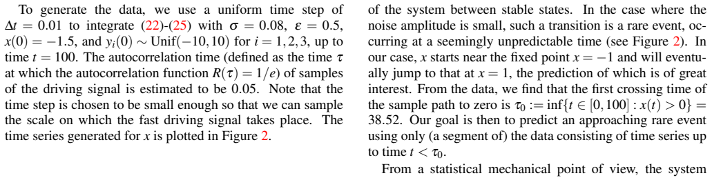
[§IV A, Eqs. (23)-(25), Algorithm III.1] For Example 1, the Lorenz-63 fast subsystem evolves on the time scale ε²=0.25, so its Lyapunov time in the slow time variable is roughly 0.28 time units; the claimed lead time of 1.62 time units is therefore about 5-6 Lyapunov times. The closed-loop ESN forecast of f in step S2 is likely far beyond the pointwise predictability horizon of the chaotic driver. Please report the ESN's actual forecast error for f on the prediction interval and explain why the integrated trajectory x still matches the target path; alternatively, state explicitly that only statistical fidelity is aimed at and adjust the comparison accordingly.
[§II, Eq. (5)] The extraction step assumes exact knowledge of the force field F, as stated in Section II. Any model error in F is converted directly into noise or bias in the training target and propagates through steps S2-S3. The paper provides no sensitivity or error analysis, so it is unclear how much error in F can be tolerated. An explicit quantification of tolerable model error, or a clear restriction of the central claim to exactly known F, is needed.
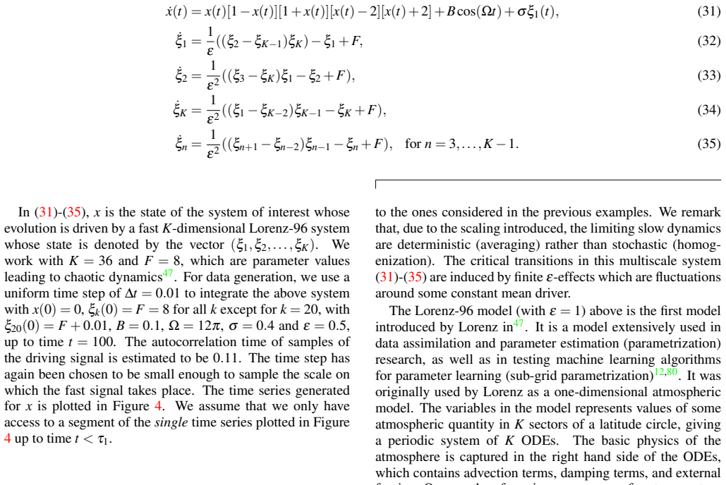
[§IV C, Table VII] In Example 3, the method succeeds in only one of the four training/validation configurations displayed (Figure 1a), a fact the authors acknowledge. This honesty is welcome, but it significantly limits the support for the paper's general claim that the method works for systems 'ranging from low dimensional to high dimensional.' The strong dependence on the tiny validation sets (Nv=5 and Nv=8) also suggests that the reported success may be fragile; please report results over the full hyperparameter grid and over multiple independent data-generation runs.
[§IV A, Results and discussion] The text asserts that prediction results of comparable quality can be obtained using a shorter trajectory starting at tinit>0 and states that this "can indeed be supported by numerical experiments," but no such experiments are shown. Either add the supporting results or remove the assertion.

minor comments (5)

[Throughout] There are several typographical errors, including "therreby" in Section I, "not suprisingly" in Section IV A, and unmatched parentheses in Eqs. (22) and (24).
[Abstract and Conclusion] The abstract's phrase "at least several numerical time steps in advance" is much weaker than the concrete 162- and 216-step claims made later; please state the quantitative claims consistently.
[Tables I-VII] Because the figures are embedded in tables without explicit axis labels or clear legends in the text, it is difficult to verify the claimed confidence-interval coverage; please provide larger, labeled figures or a separate figure file.
[Appendix] The validation set sizes (Nv=4,5,8,10,20) are extremely small, which makes the validation RMSE a noisy estimate of out-of-sample error; the paper should discuss the reliability of model selection with such small validation windows.
[§IV A] The statement that the second transition near t=71 would be predicted "confidently" if more training data were available is unsupported by any experiment; please either provide the result or soften the claim.

Circularity Check

0 steps flagged · score 0.0 of 10

No significant circularity: the transition target is out-of-sample and never enters training; the pipeline is self-contained.

full rationale

The central claim is that the extract-predict-integrate pipeline (Algorithm III.1, Eq. (5), ESN/DESN forecasting, then forward integration) can forecast a rare crossing from slow-variable data with known force field F. Checking the derivation chain, the target transition enters only as the out-of-sample test set; the ESN is trained on the extracted fast signal f(t_i) over the accessible interval, and the crossing time is not used in the training loss (Eq. (20)) or in the validation-based model selection described in the Appendix. The future x is obtained by integrating dx/dt = F(x,t) + predicted f with a Runge-Kutta scheme, not by fitting to the observed crossing. The known-F assumption (Section II) is explicitly stated, and Eq. (5) is a direct algebraic residual computation, so the forecast of f is a genuine out-of-sample time series prediction rather than a rearrangement of the target. The self-citations (refs. 1, 20, 27) motivate the problem, e.g., ref. 27 is cited as 'the main motivation of this paper,' but they do not supply the extraction formula, the reservoir computing step, or the numerical integration, and no uniqueness theorem or ansatz is imported from prior author work. The skeptical concern about Lyapunov horizons is a correctness, robustness, or generalization issue of the empirical claim, not a circularity: the paper may overstate skill on a single realization, but that does not reduce the prediction to its inputs. Accordingly, no circular step can be exhibited, and the score is 0.

Assumptions & free parameters 15 free parameters · 3 assumptions · 0 invented entities

The method introduces no new physical entities. It relies on standard domain assumptions about the slow-fast structure, exact knowledge of F, and empirical learnability of the fast signal, plus a set of tunable hyperparameters that are selected on a validation set.

free parameters (15)

reservoir size nx0 (Example 1) = 600 to 740 (grid search)
Tuned on validation set to minimize RMSE; central to ESN memory capacity.
desired spectral radius rho_des (Example 1) = 0.7
Fixed hyperparameter controlling the echo state property; not optimized.
sparsity r0 (Example 1) = 0.1
Fixed hyperparameter for reservoir connectivity.
noise intensity nu (Example 1) = 0.001
Regularization during reservoir sampling.
reservoir sizes nxi (Example 2) = 100 to 300 per layer (grid search)
Tuned on validation set for the 3-layer DESN.
desired spectral radii (Example 2) = 0.6, 0.7, 0.8 per layer
Fixed per layer.
sparsity (Example 2) = 0.05 per layer
Fixed.
noise intensity (Example 2) = 0.003
Fixed.
reservoir size nx0 (Example 3) = 500 to 700 (grid search)
Tuned on validation set.
desired spectral radius (Example 3) = 0.95
Fixed.
sparsity (Example 3) = 0.1
Fixed.
noise intensity (Example 3) = 0.003
Fixed.
number of layers L = 0 (Examples 1 and 3), 2 (Example 2)
Architecture choice; deeper network needed for multiscale fast driver in Example 2.
validation set size Nv = 10/20 (Example 1), 4/8 (Example 2), 5/8 (Example 3)
Model selection split; results depend on Nv.
confidence interval width for ensemble filtering = 8 standard deviations
Arbitrary threshold chosen to filter ensemble outliers.

assumptions (3)

domain assumption The observed slow data x(t) are generated by a slow-fast system of the form (2)-(3) with known deterministic force field F.
Section II states this family and assumes F is exactly known; if F is misspecified, the extraction in Eq. (5) is biased.
domain assumption The fast driving signal f is learnable and predictable by an echo state network from its past samples.
The method's success depends on ESN generalization; the paper cites universal approximation but does not prove it for these signals, and Example 3 shows the assumption can fail.
domain assumption Finite-difference extraction in Eq. (5) with step dt approximates the fast signal accurately enough for training.
The paper acknowledges extraction errors but provides no error bound; errors accumulate through steps S2 and S3.

how reviews work

0 comments

Cite this review

Pith. "Pith review of Predicting Critical Transitions in Multiscale Dynamical Systems Using Reservoir Computing." pith.science (2026). https://pith.science/paper/MMDHYHN7

@misc{pith2026190803771,
  author       = {Pith},
  title        = {Pith review of: Predicting Critical Transitions in Multiscale Dynamical Systems Using Reservoir Computing},
  year         = {2026},
  howpublished = {\url{https://pith.science/paper/MMDHYHN7}},
  note         = {Machine review of arXiv:1908.03771}
}

read the original abstract

We study the problem of predicting rare critical transition events for a class of slow-fast nonlinear dynamical systems. The state of the system of interest is described by a slow process, whereas a faster process drives its evolution and induces critical transitions. By taking advantage of recent advances in reservoir computing, we present a data-driven method to predict the future evolution of the state. We show that our method is capable of predicting a critical transition event at least several numerical time steps in advance. We demonstrate the success as well as the limitations of our method using numerical experiments on three examples of systems, ranging from low dimensional to high dimensional. We discuss the mathematical and broader implications of our results.

Figures

Figures reproduced from arXiv: 1908.03771 by the authors.

**Figure 3.** FIG. 3 [PITH_FULL_IMAGE:figures/full_fig_p011_3.png] view at source ↗

**Figure 4.** FIG. 4 [PITH_FULL_IMAGE:figures/full_fig_p015_4.png] view at source ↗

Discussion (0). Continue with ORCID to comment.

Reference graph

Works this paper leans on

15 extracted references · 12 canonical work pages

[1]

A GARWAL AND J

1S. A GARWAL AND J. S. W ETTLAUFER , Maximal stochastic transport in the Lorenz equations, Physics Letters A, 380 (2016), pp. 142–146. 2L. A RNOLD , Hasselmann′s program revisited: the analysis of stochasticity in deterministic climate models , in Stochastic Climate Models, Springer, 2001, pp. 141–157. 3P. A SHWIN , S. W IECZOREK , R. V ITOLO , AND P. C O...

work page 2016
[4]

Discrete-time signatures and randomness in reservoir computing

14G. C ARLEO , I. C IRAC , K. C RANMER , L. D AUDET , M. S CHULD , N. T ISHBY , L. V OGT-MARANTO , AND L. Z DEBOROVÁ , Machine learn- ing and the physical sciences , Reviews of Modern Physics, 91 (2019), p. 045002. 15A. C HATTOPADHYAY, P. H ASSANZADEH , AND D. S UBRAMANIAN , Data-driven predictions of a multiscale Lorenz 96 chaotic system using machine-le...

work page Pith review arXiv 2019
[223]

25L. P. G ARCÍA , J. D. P ÉREZ , G. V OLPE , A. V. A RZOLA , AND G. VOLPE , High-performance reconstruction of microscopic force ﬁelds from Brown- ian trajectories, Nature Communications, 9 (2018), p

work page 2018
[503]

EISENMAN AND J

20I. EISENMAN AND J. S. W ETTLAUFER , Nonlinear threshold behavior dur- ing the loss of Arctic sea ice, Proceedings of the National Academy of Sci- ences, 106 (2009), pp. 28–32. 21E. F ORGOSTON AND R. O. M OORE , A primer on noise-induced transi- tions in applied dynamical systems , SIAM Review, 60 (2018), pp. 969–

work page 2009
[865]

Risk bounds for reservoir computing

27L. G IORGINI , S. L IM, W. M OON , AND J. W ETTLAUFER , Precursors to rare events in stochastic resonance, EPL (Europhysics Letters), 129 (2020), p. 40003. 28D. G IVON , R. K UPFERMAN , AND A. S TUART , Extracting macroscopic dynamics: model problems and algorithms , Nonlinearity, 17 (2004), p. R55. 29L. G ONON , L. G RIGORYEVA , AND J.-P. O RTEGA , Ris...

work page Pith review arXiv 2020
[1009]

G ALLICCHIO AND A

22C. G ALLICCHIO AND A. M ICHELI , Deep echo state network (deepesn): a brief survey, arXiv preprint arXiv:1712.04323, (2017). 23C. G ALLICCHIO AND S. S CARDAPANE , Deep randomized neural net- works, in Recent Trends in Learning From Data, Springer, 2020, pp. 43–68. 24L. G AMMAITONI , P. HÄNGGI , P. JUNG , AND F. MARCHESONI , Stochas- tic resonance, Revie...

arXiv 2017
[1361]

M ITCHELL AND G

57L. M ITCHELL AND G. A. G OTTWALD , Data assimilation in slow–fast sys- tems using homogenized climate models , Journal of the Atmospheric Sci- ences, 69 (2012), pp. 1359–1377. 58Doing so will usually, but not always, ensure that the resulting network satisﬁes the echo state property38. 59R. P ASCANU , C. G ULCEHRE , K. C HO, AND Y. B ENGIO , How to con-...

arXiv 2012
[1996]

48Z. L U, B. R. H UNT, AND E. O TT, Attractor reconstruction by machine learning, Chaos: An Interdisciplinary Journal of Nonlinear Science, 28 (2018), p. 061104. 49M. L UKOŠEVI ˇCIUS , A practical guide to applying echo state networks , in Neural Networks: Tricks of the Trade, Springer, 2012, pp. 659–686. 50M. L UKOŠEVI ˇCIUS AND H. J AEGER , Reservoir co...

work page 2018

Show all 15 references

[2002]

J AEGER AND H

39H. J AEGER AND H. H AAS, Harnessing nonlinearity: predicting chaotic systems and saving energy in wireless communication, Science, 304 (2004), 20 pp. 78–80. 40D. T. K APLAN AND L. G LASS , Coarse-grained embeddings of time se- ries: random walks, Gaussian random processes, a...

2004 arXiv
[2006]

B ERNER , U

10J. B ERNER , U. A CHATZ , L. B ATTÉ, L. B ENGTSSON , A. D. L. CÁMARA , H. M. C HRISTENSEN , M. C OLANGELI , D. R. C OLEMAN , D. C ROM- MELIN , S. I. D OLAPTCHIEV , ET AL ., Stochastic parameterization: toward a new view of weather and climate models, Bulletin of the American...

2017
[2008]

64L. M. P ECORA AND T. L. C ARROLL , Synchronization of chaotic sys- tems, Chaos: An Interdisciplinary Journal of Nonlinear Science, 25 (2015), p. 097611. 65M. R AISSI , P. PERDIKARIS , AND G. E. K ARNIADAKIS , Physics informed deep learning (part I): data-driven solutions of ...

2015 arXiv
[2016]

32G. A. G OTTWALD AND I. M ELBOURNE , Homogenization for deter- ministic maps and multiplicative noise , Proceedings of the Royal Soci- ety A: Mathematical, Physical and Engineering Sciences, 469 (2013), p. 20130201. 33L. G RIGORYEVA AND J.-P. O RTEGA , Echo state networks are...

2013
[2019]

B ECK, Brownian motion from deterministic dynamics, Physica A: Sta- tistical Mechanics and its Applications, 169 (1990), pp

5C. B ECK, Brownian motion from deterministic dynamics, Physica A: Sta- tistical Mechanics and its Applications, 169 (1990), pp. 324–336. 6Y. BENGIO ET AL ., Learning deep architectures for AI , Foundations and Trends® in Machine Learning, 2 (2009), pp. 1–127. 7R. B ENZI , G. ...

1990
[4950]

53M. C. M ACKEY AND M. T YRAN -KAMI ´NSKA , Deterministic Brownian motion: the effects of perturbing a dynamical system by a chaotic semi- dynamical system, Physics Reports, 422 (2006), pp. 167–222. 54G. M ANJUNATH AND H. J AEGER , Echo state property linked to an input: explo...

2006
[5166]

G ASPARD , M

26P. G ASPARD , M. B RIGGS , M. F RANCIS , J. S ENGERS , R. G AMMON , J. R. D ORFMAN , AND R. C ALABRESE , Experimental evidence for mi- 19 FIG. 5: A schematic summarizing the workﬂow of our data-driven method for rare event prediction. In the schematic below, (S1)-(S3) denote...

1998

Pith tools

Reviewed August 14, 2026 · model on record in the stance chip above.

[1] [1]

A GARWAL AND J

1S. A GARWAL AND J. S. W ETTLAUFER , Maximal stochastic transport in the Lorenz equations, Physics Letters A, 380 (2016), pp. 142–146. 2L. A RNOLD , Hasselmann′s program revisited: the analysis of stochasticity in deterministic climate models , in Stochastic Climate Models, Springer, 2001, pp. 141–157. 3P. A SHWIN , S. W IECZOREK , R. V ITOLO , AND P. C O...

work page 2016

[2] [4]

Discrete-time signatures and randomness in reservoir computing

14G. C ARLEO , I. C IRAC , K. C RANMER , L. D AUDET , M. S CHULD , N. T ISHBY , L. V OGT-MARANTO , AND L. Z DEBOROVÁ , Machine learn- ing and the physical sciences , Reviews of Modern Physics, 91 (2019), p. 045002. 15A. C HATTOPADHYAY, P. H ASSANZADEH , AND D. S UBRAMANIAN , Data-driven predictions of a multiscale Lorenz 96 chaotic system using machine-le...

work page Pith review arXiv 2019

[3] [223]

25L. P. G ARCÍA , J. D. P ÉREZ , G. V OLPE , A. V. A RZOLA , AND G. VOLPE , High-performance reconstruction of microscopic force ﬁelds from Brown- ian trajectories, Nature Communications, 9 (2018), p

work page 2018

[4] [503]

EISENMAN AND J

20I. EISENMAN AND J. S. W ETTLAUFER , Nonlinear threshold behavior dur- ing the loss of Arctic sea ice, Proceedings of the National Academy of Sci- ences, 106 (2009), pp. 28–32. 21E. F ORGOSTON AND R. O. M OORE , A primer on noise-induced transi- tions in applied dynamical systems , SIAM Review, 60 (2018), pp. 969–

work page 2009

[5] [865]

Risk bounds for reservoir computing

27L. G IORGINI , S. L IM, W. M OON , AND J. W ETTLAUFER , Precursors to rare events in stochastic resonance, EPL (Europhysics Letters), 129 (2020), p. 40003. 28D. G IVON , R. K UPFERMAN , AND A. S TUART , Extracting macroscopic dynamics: model problems and algorithms , Nonlinearity, 17 (2004), p. R55. 29L. G ONON , L. G RIGORYEVA , AND J.-P. O RTEGA , Ris...

work page Pith review arXiv 2020

[6] [1009]

G ALLICCHIO AND A

22C. G ALLICCHIO AND A. M ICHELI , Deep echo state network (deepesn): a brief survey, arXiv preprint arXiv:1712.04323, (2017). 23C. G ALLICCHIO AND S. S CARDAPANE , Deep randomized neural net- works, in Recent Trends in Learning From Data, Springer, 2020, pp. 43–68. 24L. G AMMAITONI , P. HÄNGGI , P. JUNG , AND F. MARCHESONI , Stochas- tic resonance, Revie...

arXiv 2017

[7] [1361]

M ITCHELL AND G

57L. M ITCHELL AND G. A. G OTTWALD , Data assimilation in slow–fast sys- tems using homogenized climate models , Journal of the Atmospheric Sci- ences, 69 (2012), pp. 1359–1377. 58Doing so will usually, but not always, ensure that the resulting network satisﬁes the echo state property38. 59R. P ASCANU , C. G ULCEHRE , K. C HO, AND Y. B ENGIO , How to con-...

arXiv 2012

[8] [1996]

48Z. L U, B. R. H UNT, AND E. O TT, Attractor reconstruction by machine learning, Chaos: An Interdisciplinary Journal of Nonlinear Science, 28 (2018), p. 061104. 49M. L UKOŠEVI ˇCIUS , A practical guide to applying echo state networks , in Neural Networks: Tricks of the Trade, Springer, 2012, pp. 659–686. 50M. L UKOŠEVI ˇCIUS AND H. J AEGER , Reservoir co...

work page 2018