Automated classification of plasma regions using 3D particle energy distributions

Ahmad Lalti; Andrew P. Dimmock; Andrey Divin; Gian Luca Delzanno; Levon Avanov; Pawel Herman; Stefano Markidis; Steven W.D. Chien; Sven Anderzen; Vyacheslav Olshevsky

REVIEW 3 major objections 4 minor 18 references

Automated classification of plasma regions using 3D particle energy distributions

T0 review · 3 major / 4 minor · reviewed 2026-08-14 · deepseek-v4-flash

Challenge this review Re-run · record.json Download PDF Read on arXiv ↗ Review JSON

Pith's one-line read A 3D convolutional neural network trained on single ion-energy snapshots classifies the four dayside plasma regions crossed by MMS with more than 98% accuracy, and its low-confidence outputs flag boundary regions such as the bow shock.

desk verdict Solid, reproducible CNN for MMS plasma region classification, with aggregate accuracy claims that overstate per-class IF performance and an archive-scale application that remains a proof of concept. read the letter →

arxiv 1908.05715 v4 pith:P2OTOO4J submitted 2019-08-15 physics.space-ph cs.LGeess.IV

Vyacheslav Olshevsky , Yuri V. Khotyaintsev , Ahmad Lalti , Andrey Divin , Gian Luca Delzanno , Sven Anderzen , Pawel Herman , Steven W.D. Chien

show 3 more authors

Levon Avanov Andrew P. Dimmock Stefano Markidis

This is my paper · ORCID

classification physics.space-phcs.LGeess.IV

keywords plasmaregionclassificationconvolutionalneuralnetworkionskymapsMagnetosphericMultiscalemissionforeshockmagnetosheathbowshockdetectionmagnetopause

verification ladder T0 review T1 audit T2 compute T3 formal

The pith

A machine-rendered reading of the paper's core claim, the machinery that carries it, and where it could break.

The reading

This paper sets out to show that the four main dayside plasma regions crossed by a spacecraft near Earth—solar wind, ion foreshock, magnetosheath, and magnetosphere—can be recognized automatically from a single three-dimensional snapshot of ion velocities and energies. The authors train a 3D convolutional neural network on human-labeled ion distributions from one month of MMS observations and test it on a different month, so the network must generalize rather than memorize. The reported result is agreement with human labels above 98% for both cross-validations. If correct, the method would let the full MMS archive be sorted into scientifically meaningful regions without manual surveying, and low-confidence predictions would draw attention to boundary layers such as the bow shock and magnetopause.

What carries the argument

The central object is the 3D convolutional neural network applied directly to the array of ion phase-space densities, with axes for energy, polar angle, and azimuthal angle. Preprocessing replaces zero-count bins with the smallest nonzero value, takes logarithms, normalizes each sample, and wraps the polar-angle axis so the solar-wind beam falls in the center. The network uses two 3D convolution layers with strided filters, a 3D max-pooling layer, and two fully connected layers, ending in four probabilities that sum to one. A dominant probability is the classification; the absence of a dominant probability is interpreted as a mixed or boundary plasma, which is the mechanism that lets the same model flag bow-shock and magnetopause crossings.

What would settle it

Take the two trained models and test them on a third, independently labeled month of MMS data or on the other MMS spacecraft, and compare their boundary detections with crossings identified from magnetic-field and plasma parameters; if per-class accuracy on the ion foreshock falls well below the human-label agreement rate, or if the flagged shock crossings disagree with field-based identifications, the generalization claim fails.

Watch

Extended reading notes

Core claim

The central claim is that a single 32 by 16 by 32 ion energy distribution recorded by the FPI/DIS instrument carries enough information to identify which of four dayside plasma regions the spacecraft is in. A 3D convolutional neural network trained on roughly 25,000 human-labeled samples from one month assigns the correct region for more than 98% of samples from a different month, using no time history and no magnetic-field input. The network's four output probabilities also serve as a boundary detector: when no class reaches a high probability, the sample is treated as a mixed plasma population, and rapid probability transitions between magnetosheath and solar wind or foreshock are used to mark bow-shock crossings.

Load-bearing premise

The human-labeled samples are treated as the ground truth for the four regions, so the reported accuracy measures agreement with those labels rather than with an independent physical classification.

Editorial extensions

If this is right

The full MMS dayside archive can be classified sample by sample, enabling large statistical surveys of when and where each plasma region occurs.
Bow-shock crossings can be detected automatically from probability transitions; the paper reports that all 12 crossings in a test interval were identified.
The same low-confidence mechanism can be applied to magnetopause crossings and to searches for mixed populations where reconnection is likely.
Because the input is only the ion distribution, the approach could extend to other spacecraft or particle instruments whenever their region signatures appear in the distributions.

Reading between the lines

Editorial extensions of the paper, not claims the author makes directly.

Agreement with human labels is not the same as physical truth; an independent test against boundary identifications from magnetic field and plasma parameters would clarify how much of the reported accuracy reflects real physics rather than label replication.
The model's probability scores define a continuous boundary layer whose thickness could be used as a data-driven measure of how sharply the bow shock and magnetopause respond to changing solar-wind conditions.
Because each sample is classified independently, the pipeline could plausibly run in near-real time after downlink, or even onboard, to flag boundary crossings for targeted burst-mode data collection.

Share X Bluesky LinkedIn Reddit HN

Signed reviews

No signed human review yet.

Editorial analysis

A structured set of objections, weighed in public.

Desk editor's note, referee report, and a circularity audit.

Desk Editor's Note

read the letter

Here's the short version: this is a legitimate, reproducible machine-learning paper that does what it says for a four-class labeling problem, and the authors are honest about the harder parts. The genuinely new thing is the direct use of 3D FPI/DIS ion sky maps as CNN input for classifying solar wind, ion foreshock, magnetosheath, and magnetosphere, instead of the feature-vector Bayesian/LSTM approaches in Piatt (2019) and Argall et al. (2020). The cross-month validation on ~470k labeled samples is solid: two models, swap training and validation months, per-class confusion matrices, public code and data. They even report the ugly number: per-class IF accuracy is 83.8% and 93.4%, and they acknowledge that human labelers themselves confuse IF with SW (Section 4.1). That is exactly the right way to report.

Soft spots, in proportion. The >98% accuracy is aggregate and dominated by easy SW/MSH/MSP classes; the abstract and Key Points lead with that number, and the IF caveat gets pushed to Section 4. That matters for the intended use, because IF is a region scientists care about. Also, the accuracy measures agreement with two months of human labels, not an independent physical ground truth. The whole-archive claim in the abstract outruns the evidence: the only out-of-sample physical check is the single November 2018 bow-shock event in Section 4.2, and the shock detection rule (transition within a window) is defined in a post-hoc way with hand-chosen parameters. The paper calls this 'preliminary results,' which is fair, but then the abstract should not say the technique 'can be used for classification of the whole MMS database' as if it were established.

The citation pattern is fine. The PCA section is a bit decorative but harmless. The baseline comparison is missing -- no direct run of Piatt or Argall on the same data -- but the authors are not claiming to beat them on identical footing.

Bottom line: the core result, a CNN that reproduces human regional labels on an unseen month from raw sky maps, holds up. The boundary-detection and archive-wide claims need more validation. This deserves peer review -- a good referee could help reframe the claims and add a per-class breakdown in the abstract. I'd take it to reading group as an example of how to do a solid, self-aware ML application in space physics.

Referee Report

3 major / 4 minor

Summary. The paper presents a 3D convolutional neural network that classifies MMS/Fast Plasma Investigation (FPI) Dual Ion Spectrometer (DIS) ion energy distributions into four dayside plasma regions: solar wind (SW), ion foreshock (IF), magnetosheath (MSH), and magnetosphere (MSP). The input is a single 32×16×32 energy/angle array, and the network outputs class probabilities. The authors label two months (November and December 2017) of MMS1 data by hand, train one model per month on balanced subsets, and cross-validate each model against the other month, reporting aggregate accuracies of 98.4% and 98.9%. They further propose that low-confidence predictions indicate mixed plasma regions and demonstrate a shock-crossing detection scheme on a single November 2018 event, concluding that the method can be applied to the whole MMS database.

Significance. If the claims were fully supported, the paper would provide a useful, fast, end-to-end tool for automatically labeling dayside plasma regions in the MMS archive, which could benefit statistical studies of the bow shock, magnetopause, and reconnection. The strengths of the paper are its clearly described architecture and preprocessing, the large labeled dataset, the cross-month validation with confusion matrices, and the public release of code and labeled data, which support reproducibility. The main limitation is that the reported accuracy measures agreement with the authors' own human interval labels rather than with an independent physical ground truth, and the broader applicability claims rest on a single out-of-sample event.

major comments (3)

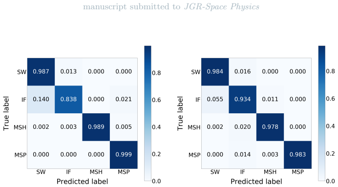
[Section 2.1, Table 1, and Figure 6] The headline accuracy of >98% is computed against human interval labels, not against an independent physical classification, and the aggregate number is dominated by the three easier classes: IF constitutes only 8.9–10.7% of the labeled samples, while the per-class IF accuracies in Figure 6 are 83.8% and 93.4%. Please report per-class precision and recall, provide confidence intervals for the aggregate accuracy, and explicitly state in the abstract and conclusions that the metric is agreement with the authors' labeling scheme, as Section 4.1 itself acknowledges that IF samples are often mislabeled as SW even by humans.
[Section 4.2 and Conclusions] The claims that the method can be used to detect bow-shock and magnetopause crossings and to classify the whole MMS database are not supported by the presented evidence: the only out-of-sample demonstration is a single November 2018 event with 12 hand-verified crossings, and the shock-detection rule depends on unspecified thresholds such as a transition on a 'set period'. Please provide a quantitative evaluation over multiple crossings and months, or rescope the conclusions to state that this is a feasibility demonstration rather than a validated whole-archive capability.
[Sections 3.1 and 4.1] The definitions of 'clean' versus 'mixed' predictions via top-probability thresholds of 0.7 and 0.5 are introduced without justification or sensitivity analysis, and the 0.04% of samples flagged as mixed is not validated against independently identified boundary crossings. Please quantify how the thresholds affect the reported mixed-region and shock-crossing results, or clearly label these thresholds as provisional and heuristic.

minor comments (4)

[Section 2.2, step 4] There is an axis-indexing inconsistency: the array dimensions are described as energy, polar angle θ, and azimuthal angle φ, so wrapping the solar-wind beam to the center should be along the second axis (θ), not the 'third axis' as stated in step 4; please verify and correct the wording.
[Section 3.1 and Table 2] The text states that about 12% or 1/8 of the labeled samples were used for training, but Table 2 shows 25,532 of 278,110 samples for November (about 9.2% of all samples and 10.8% of non-Unknown samples) and 25,275 of 191,168 for December (about 13.2% of all samples); please reconcile these numbers or clarify the selection procedure.
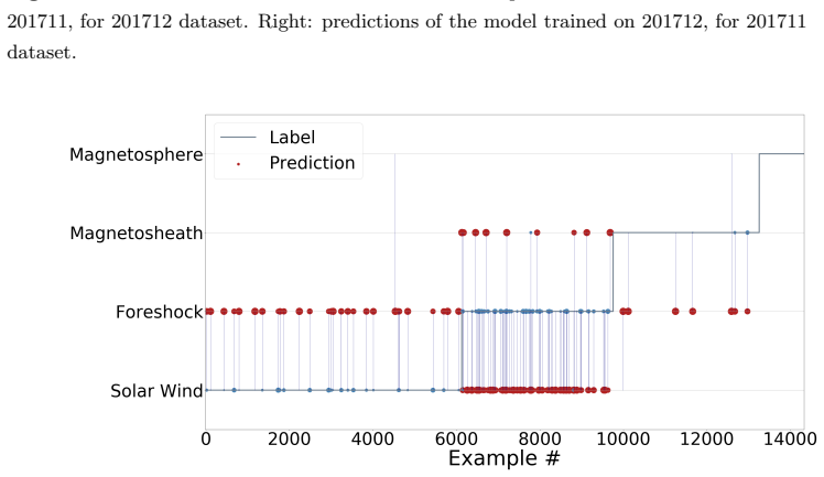
[Figure 7 caption] The caption states that the grey line is the reference human-made label and that red and blue circles represent wrong and second-most-probable predictions, but it is not clear what the sizes of the circles encode beyond probability; please clarify the figure's visual encoding.
[Affiliations] The affiliation of A. Divin is spelled 'St. Petersbourgh', which should be corrected to 'St. Petersburg'.

Circularity Check

0 steps flagged · score 0.0 of 10

No circularity: the 98% accuracy is a measured agreement with human labels in a supervised-learning setup, not a quantity forced by construction, and the bow-shock application is an independent downstream use of the trained classifier.

full rationale

The paper's central claim is that a 3D CNN trained on human-labeled MMS FPI/DIS ion distributions can classify four dayside plasma regions with >98% cross-month accuracy. This is a standard supervised-learning benchmark: the human labels (Section 2.1) are external ground truth, the model is trained on a subset of one month's labels, and the reported accuracy is computed on held-out labels from the other month (Section 4). There is no fitted parameter that is subsequently renamed as a prediction, and no equation in the paper defines the predicted class probabilities in terms of the labels or of the accuracy metric. The acknowledged difficulty of classifying ion foreshock, which is often mislabeled even by humans, is a limitation in the ground-truth quality, not a circular derivation. The bow-shock detection procedure (Section 4.2) takes the trained model's probability outputs and defines crossings as fast probability transitions; this is an application of the classifier, and its illustration on an independent 2018 event is an out-of-sample check rather than a reconstruction of the training input. The whole-archive generalization claim is an extrapolation beyond the validated two months, but that is a scope or evidence-strength concern, not circularity. The derivation chain is self-contained: data preprocessing, CNN training, cross-validation, and downstream event detection are sequential and do not assume the result they claim to produce.

Assumptions & free parameters 4 free parameters · 4 assumptions · 0 invented entities

The paper makes an empirical machine learning claim; its free parameters are the trained network weights and hand-chosen thresholds. No new physical entities are introduced. The core assumptions are the validity of human labels and the representativeness of two months of data.

free parameters (4)

CNN trainable weights = Learned from approximately 25,000 training samples per model
The classifier's predictions are entirely determined by these fitted weights, trained as described in Section 3.2.
Top-probability threshold for mixed regions = 0.5
Section 4.1 defines samples with top score below 0.5 as mixed or boundary regions; the threshold is chosen by hand and not optimized or independently validated.
Training data selection fractions = Approximately 1/8 per class, adjusted for rare classes
Section 3.1: random selection coefficients are chosen by hand to balance the training set; exact coefficients are not reported.
Shock-crossing detection time window = Not specified
Section 4.2 defines a crossing as a probability change 'within a set period' but the period is never quantified, so the detector is not fully specified.

assumptions (4)

domain assumption Human-labeled classes are the ground truth for the four plasma regions.
Section 2.1 describes interactive labeling; the reported accuracy is agreement with these labels, so label quality bounds the significance of the accuracy claim.
domain assumption The 32x16x32 ion phase-space distributions contain enough information to separate the four regions.
Section 2 and Figure 1 argue that each region has distinct features; the trained network's performance supports this, but it is assumed at the outset.
domain assumption Samples from November and December 2017 are representative of the MMS dayside database.
Section 4 uses the two months for training and cross-validation; Section 4.2 applies the models to the whole archive from 2015 without revalidation, assuming the learned mapping is stationary.
domain assumption Wrapping the array by 16 elements along the azimuthal axis centers the solar wind beam.
Section 2.2 step 4; the text refers to the third axis as theta, but the third array axis is azimuthal angle phi, a minor inconsistency in preprocessing.

how reviews work

0 comments

Cite this review

Pith. "Pith review of Automated classification of plasma regions using 3D particle energy distributions." pith.science (2026). https://pith.science/paper/P2OTOO4J

@misc{pith2026190805715,
  author       = {Pith},
  title        = {Pith review of: Automated classification of plasma regions using 3D particle energy distributions},
  year         = {2026},
  howpublished = {\url{https://pith.science/paper/P2OTOO4J}},
  note         = {Machine review of arXiv:1908.05715}
}

read the original abstract

We investigate the properties of the ion sky maps produced by the Dual Ion Spectrometers (DIS) from the Fast Plasma Investigation (FPI). We have trained a convolutional neural network classifier to predict four regions crossed by the MMS on the dayside magnetosphere: solar wind, ion foreshock, magnetosheath, and magnetopause using solely DIS spectrograms. The accuracy of the classifier is >98%. We use the classifier to detect mixed plasma regions, in particular to find the bow shock regions. A similar approach can be used to identify the magnetopause crossings and reveal regions prone to magnetic reconnection. Data processing through the trained classifier is fast and efficient and thus can be used for classification for the whole MMS database.

Figures

Figures reproduced from arXiv: 1908.05715 by the authors.

**Figure 1.** Volume rendering of the logarithm of the ion phase space density for four typical observations. In each panel, x corresponds to the energy bin, y to θ, and z - to φ. The axes are denoted in the lower left corner of each panel with red (x), yellow (y), green (z). a) Solar Wind; b) Ion foreshock; c) Magnetosheath; d) Magnetosphere. 2.1 Human-labeled datasets We have labeled 2 sets of measurements taken by the DIS on M… view at source ↗

**Figure 2.** Projection of the human-labeled 201711 dataset on the two first PCs. Each circle represents one sample: SW (grey), MSP (green), MSH (blue), IF (red), UNK (black). 2 first components are of interest. This array contains the ‘projection’ of each n-size measurement vector on the first 2 PC basis vectors containing most variance of the dataset. We have computed the PCA over the human-labeled datasets ( [PITH_FULL_IMAG… view at source ↗

**Figure 3.** Observations on 2017.11.15 12:00 – 14:00. a) log10 of the energy distribution integrated over φ, θ. White pixels at high energy indicate no counts detected at higher energies in the colder solar wind which we replace with a very small value. b) Blue, green, red: Bx,GSM , By,GSM , Bz,GSM . c) Left axis, light grey: projection of the data on the first PC; right, axis, dark grey: projection of the data on the second P… view at source ↗

Figures from the paper (6 more)

**Figure 4.** Figure 4: a, b) Volume rendering and slice cuts through the first PC computed from the human-labeled dataset, reshaped to 32 × 16 × 32 array. Red color represents high variance, blue corresponds to low variance. c,d) Same for the second PC. all samples is used for training. The …

**Figure 5.** Figure 5: The architecture of the classifier model. & Ba, 2014) with learning rate α = 1 · 10−6 , and a categorical cross-entropy loss L = − X C i ti log (f (si)), (1) where ti is the ground-truth probability (either 1 or 0), C = 4 is the number of classes, and f (si) = e si PC …

**Figure 6.** Figure 6: Cross-validation confusion matrices. Left: predictions of the model trained on 201711, for 201712 dataset. Right: predictions of the model trained on 201712, for 201711 dataset [PITH_FULL_IMAGE:figures/full_fig_p011_6.png]

**Figure 7.** Figure 7: A typical case in which the 201711-trained model misclassifies samples from the IF region. Grey line is the reference human-made label. Red circles correspond to the wrong predictions. Blue circles represent the second most probable predictions for each mislabeled exa…

**Figure 8.** Figure 8: Predictions of the trained CNN for two months of observations, 201711 and 201712 plotted in the xGSE and yGSE coordinates. Color circles denote different regions, and the grey line shows the spacecraft trajectory. coded with blue (SW), black (IF), yellow (MSH), and red…

**Figure 9.** Figure 9: Detection of shock crossing events using the probability output of the CNN model. (a) magnetic field, (b) omni-directional ion differential energy flux (DEF), (c) probability output from the classifier, color coded with Blue being SW, black IF, yellow MSH and red MSP, …

Discussion (0). Continue with ORCID to comment.

Reference graph

Works this paper leans on

18 extracted references · 8 canonical work pages

[1]

, " * write output.state after.block = add.period write newline

ENTRY address author booktitle chapter doi edition editor eid howpublished institution journal key month note number organization pages publisher school series title type volume year label extra.label sort.label short.list INTEGERS output.state before.all mid.sentence after.sentence after.block FUNCTION init.state.consts #0 'before.all := #1 'mid.sentence...
[2]

write newline

" write newline "" before.all 'output.state := FUNCTION if.digit duplicate "0" = swap duplicate "1" = swap duplicate "2" = swap duplicate "3" = swap duplicate "4" = swap duplicate "5" = swap duplicate "6" = swap duplicate "7" = swap duplicate "8" = swap "9" = or or or or or or or or or FUNCTION n.separate 't := "" #0 'numnames := t empty not t #-1 #1 subs...
[3]

, Agarwal, A

tensorflow2015-whitepaper APACrefauthors Abadi, M. , Agarwal, A. , Barham, P. , Brevdo, E. , Chen, Z. , Citro, C. Zheng, X. APACrefauthors \ 2015 . TensorFlow : Large-Scale Machine Learning on Heterogeneous Systems. TensorFlow : Large-scale machine learning on heterogeneous systems. APACrefURL https://www.tensorflow.org/ APACrefURL Software available from...

work page 2015
[4]

, Small, C R

Argall:etal:2020 APACrefauthors Argall, M R. , Small, C R. , Piatt, S. , Breen, L. , Petrik, M. , Kokkonen, K. Burch, J L. APACrefauthors \ 2020 . MMS SITL Ground Loop: Automating the Burst Data Selection Process Mms sitl ground loop: Automating the burst data selection process . Frontiers in Astronomy and Space Sciences 7 54 . APACrefURL https://www.fron...

arXiv 2020
[5]

, Moore, T E

Burch:2016 APACrefauthors Burch, J L. , Moore, T E. , Torbert, R B. \ Giles, B L. APACrefauthors \ 2016 Mar 01 . Magnetospheric Multiscale Overview and Science Objectives Magnetospheric multiscale overview and science objectives . Space Science Reviews 199 1 5--21 . APACrefURL https://doi.org/10.1007/s11214-015-0164-9 APACrefURL APACrefDOI doi:10.1007/s11...

doi:10.1007/s11214-015-0164-9 2016
[6]

chollet2015keras APACrefauthors Chollet, F. \ . APACrefauthors \ 2015 . Keras. Keras. https://keras.io

work page 2015
[7]

, Lewis, W S

Fuselier:2016 APACrefauthors Fuselier, S A. , Lewis, W S. , Schiff, C. , Ergun, R. , Burch, J L. , Petrinec, S M. \ Trattner, K J. APACrefauthors \ 2016 Mar 01 . Magnetospheric Multiscale Science Mission Profile and Operations Magnetospheric multiscale science mission profile and operations . Space Science Reviews 199 1 77--103 . APACrefURL https://doi.or...

work page doi:10.1007/s11214-014-0087-x 2016
[8]

, Vines, S K

Fuselier:2017 APACrefauthors Fuselier, S A. , Vines, S K. , Burch, J L. , Petrinec, S M. , Trattner, K J. , Cassak, P A. Webster, J M. APACrefauthors \ 2017 . Large-scale characteristics of reconnection diffusion regions and associated magnetopause crossings observed by MMS Large-scale characteristics of reconnection diffusion regions and associated magne...

work page 2017

Show all 18 references

[9]

APACrefauthors \ 1933

Hotelling:1933 APACrefauthors Hotelling, H. APACrefauthors \ 1933 . Analysis of a Complex of Statistical Variables Into Principal Components Analysis of a complex of statistical variables into principal components . Journal of Educational Psychology 24 417-441,498-520

1933
[10]

APACrefauthors \ 2002

Jolliffe:2002:PCA APACrefauthors Jolliffe, I. APACrefauthors \ 2002 . Principal Component Analysis Principal component analysis . Springer . APACrefURL https://books.google.se/books?id=\_olByCrhjwIC APACrefURL

2002
[11]

kingma:2014 APACrefauthors Kingma, D P. \ Ba, J. APACrefauthors \ 2014 . Adam: A method for stochastic optimization Adam: A method for stochastic optimization . arXiv preprint arXiv:1412.6980

2014 arXiv
[12]

, Bengio , Y

Lecun:Yann:Bengio:2015 APACrefauthors LeCun , Y. , Bengio , Y. \ Hinton , G. APACrefauthors \ 2015 May . Deep learning Deep learning . Nature 521 7553 436-444 . APACrefDOI doi:10.1038/nature14539 APACrefDOI

2015 doi
[13]

\ Scherer , S

Maturana:Scherer:2015 APACrefauthors Maturana , D. \ Scherer , S. APACrefauthors \ 2015 Sep. . VoxNet: A 3D Convolutional Neural Network for real-time object recognition Voxnet: A 3d convolutional neural network for real-time object recognition . 2015 IEEE/RSJ International Co...

2015
[14]

APACrefauthors \ 1901

Pearson:1901:PCA APACrefauthors Pearson, K. APACrefauthors \ 1901 . LIII. On lines and planes of closest fit to systems of points in space Liii. on lines and planes of closest fit to systems of points in space . The London, Edinburgh, and Dublin Philosophical Magazine and Jour...

1901 doi
[15]

, Varoquaux, G

scikit-learn APACrefauthors Pedregosa, F. , Varoquaux, G. , Gramfort, A. , Michel, V. , Thirion, B. , Grisel, O. Duchesnay, E. APACrefauthors \ 2011 . Scikit-learn: Machine Learning in P ython Scikit-learn: Machine learning in P ython . Journal of Machine Learning Research 12 ...

2011
[16]

APACrefauthors \ 2019 May

Piatt:2019arXiv APACrefauthors Piatt , S. APACrefauthors \ 2019 May . Large-Scale Statistical Survey of Magnetopause Reconnection Large-Scale Statistical Survey of Magnetopause Reconnection . arXiv e-prints arXiv:1905.11359

2019 arXiv
[17]

, Moore, T

Pollock:2016 APACrefauthors Pollock, C. , Moore, T. , Jacques, A. , Burch, J. , Gliese, U. , Saito, Y. Zeuch, M. APACrefauthors \ 2016 Mar 01 . Fast Plasma Investigation for Magnetospheric Multiscale Fast plasma investigation for magnetospheric multiscale . Space Science Revie...

2016 doi
[18]

, Anderson, B J

Russell:2016 APACrefauthors Russell, C T. , Anderson, B J. , Baumjohann, W. , Bromund, K R. , Dearborn, D. , Fischer, D. Richter, I. APACrefauthors \ 2016 Mar 01 . The Magnetospheric Multiscale Magnetometers The magnetospheric multiscale magnetometers . Space Science Reviews 1...

2016 doi

Pith tools

Reviewed August 14, 2026 · model on record in the stance chip above.

[1] [1]

, " * write output.state after.block = add.period write newline

ENTRY address author booktitle chapter doi edition editor eid howpublished institution journal key month note number organization pages publisher school series title type volume year label extra.label sort.label short.list INTEGERS output.state before.all mid.sentence after.sentence after.block FUNCTION init.state.consts #0 'before.all := #1 'mid.sentence...

[2] [2]

write newline

" write newline "" before.all 'output.state := FUNCTION if.digit duplicate "0" = swap duplicate "1" = swap duplicate "2" = swap duplicate "3" = swap duplicate "4" = swap duplicate "5" = swap duplicate "6" = swap duplicate "7" = swap duplicate "8" = swap "9" = or or or or or or or or or FUNCTION n.separate 't := "" #0 'numnames := t empty not t #-1 #1 subs...

[3] [3]

, Agarwal, A

tensorflow2015-whitepaper APACrefauthors Abadi, M. , Agarwal, A. , Barham, P. , Brevdo, E. , Chen, Z. , Citro, C. Zheng, X. APACrefauthors \ 2015 . TensorFlow : Large-Scale Machine Learning on Heterogeneous Systems. TensorFlow : Large-scale machine learning on heterogeneous systems. APACrefURL https://www.tensorflow.org/ APACrefURL Software available from...

work page 2015

[4] [4]

, Small, C R

Argall:etal:2020 APACrefauthors Argall, M R. , Small, C R. , Piatt, S. , Breen, L. , Petrik, M. , Kokkonen, K. Burch, J L. APACrefauthors \ 2020 . MMS SITL Ground Loop: Automating the Burst Data Selection Process Mms sitl ground loop: Automating the burst data selection process . Frontiers in Astronomy and Space Sciences 7 54 . APACrefURL https://www.fron...

arXiv 2020

[5] [5]

, Moore, T E

Burch:2016 APACrefauthors Burch, J L. , Moore, T E. , Torbert, R B. \ Giles, B L. APACrefauthors \ 2016 Mar 01 . Magnetospheric Multiscale Overview and Science Objectives Magnetospheric multiscale overview and science objectives . Space Science Reviews 199 1 5--21 . APACrefURL https://doi.org/10.1007/s11214-015-0164-9 APACrefURL APACrefDOI doi:10.1007/s11...

doi:10.1007/s11214-015-0164-9 2016

[6] [6]

chollet2015keras APACrefauthors Chollet, F. \ . APACrefauthors \ 2015 . Keras. Keras. https://keras.io

work page 2015

[7] [7]

, Lewis, W S

Fuselier:2016 APACrefauthors Fuselier, S A. , Lewis, W S. , Schiff, C. , Ergun, R. , Burch, J L. , Petrinec, S M. \ Trattner, K J. APACrefauthors \ 2016 Mar 01 . Magnetospheric Multiscale Science Mission Profile and Operations Magnetospheric multiscale science mission profile and operations . Space Science Reviews 199 1 77--103 . APACrefURL https://doi.or...

work page doi:10.1007/s11214-014-0087-x 2016

[8] [8]

, Vines, S K

Fuselier:2017 APACrefauthors Fuselier, S A. , Vines, S K. , Burch, J L. , Petrinec, S M. , Trattner, K J. , Cassak, P A. Webster, J M. APACrefauthors \ 2017 . Large-scale characteristics of reconnection diffusion regions and associated magnetopause crossings observed by MMS Large-scale characteristics of reconnection diffusion regions and associated magne...

work page 2017