REVIEW 4 major objections 6 minor 22 references
Structural Health Monitoring of Cantilever Beam, a Case Study -- Using Bayesian Neural Network AND Deep Learning
T0 review · 4 major / 6 minor · reviewed 2026-08-14 · deepseek-v4-flash
Pith's one-line read A four-element cantilever-beam case study reports that a Bayesian neural network, an LSTM, and a 2D CNN all predict per-element bending rigidity from raw frequency responses, with R2 scores of 0.9967, 0.9910, and 0.9862.
desk verdict Simulation-only case study shows stock neural nets hit high R² on FE beam data, but the real-SHM claims are unsupported. read the letter →
The pith
A machine-rendered reading of the paper's core claim, the machinery that carries it, and where it could break.
The reading
What carries the argument
The load-bearing object is the FE-simulated frequency-response vector: a 40,000-length concatenation of acceleration responses from nodes 5, 4, 3, and 2, with damage encoded as the four element diameters. The paper feeds this raw vector directly into three architectures. Probabilistic backpropagation (PBP) trains the Bayesian network by replacing point-estimate weights with one-dimensional Gaussians that approximate the posterior marginals. The CNN reshapes each vector to 200 by 200 and stacks convolution and pooling layers, while the LSTM treats the vector as four time steps of 10,000 frequencies. The machinery does the work of mapping damage state to response without hand-crafted features.
What would settle it
Measure frequency responses on a physical cantilever beam with known element diameters and feed them to the trained models: if the $R^2$ scores fall substantially or predicted diameters systematically drift, the simulation-to-reality transfer fails. A cheaper test is to add realistic sensor noise to the FE inputs and track $R^2$ degradation.
Extended reading notes
Core claim
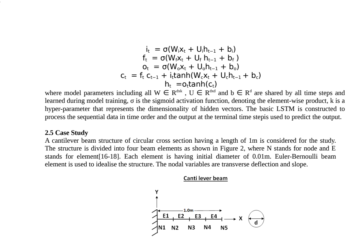
The paper reports that, on a finite-element model of a 1 m cantilever beam split into four elements, damage simulated by varying element diameters from 0.005 to 0.015 m is recoverable from raw frequency-response data. Each input is the concatenated acceleration response at four nodes over 10,000 frequencies (vector length 40,000), and each output is the four element diameters. A Bayesian multi-layer perceptron trained with probabilistic backpropagation achieves $R^2 = 0.9967$ on held-out data, an LSTM achieves $R^2 = 0.9910$, and a 2D CNN achieves $R^2 = 0.9862$. The paper takes these scores, all close to 1, as evidence that the three architectures are effective for vibration-based SHM and can predict bending rigidity with acceptable error. It also uses gradient visualization to argue that lower modes identify damage near the fixed end and higher modes identify damage near the free end.
Load-bearing premise
The whole argument rests on treating the finite-element-generated frequency responses as if they were real sensor measurements, because the same simulation supplies both the inputs and the diameter labels with no added noise or modeling error.
Editorial extensions
If this is right
- If the reported $R^2$ values transfer beyond the simulation, structural health monitoring can run on raw vibration streams with no manual feature extraction, which the paper notes suits real-time monitoring.
- The Bayesian variant provides uncertainty over predictions, so it could flag damage states unlike any seen in training rather than silently returning a confident diameter.
- The gradient visualization suggests sensor or mode selection can be tailored by damage location: lower modes for near-fixed-end damage and higher modes for near-free-end damage.
- The same raw-signal pipeline could in principle be applied to other beam-like or plate structures, though the paper's direct evidence is limited to this four-element cantilever case.
Reading between the lines
- Beyond the paper: because the same FE model generates both inputs and labels, the reported $R^2$ partly measures how well each network inverts that specific simulator; real-world transfer would need independent validation on measured responses.
- Beyond the paper: adding sensor noise or boundary-condition variation to the FE inputs would quantify robustness, which the current study does not address.
- Beyond the paper: the LSTM's slight edge over the CNN may depend on the chosen input reshaping (four time steps of 10,000 frequencies); alternative reshape schemes could change the ranking.
Signed reviews
Editorial analysis
A structured set of objections, weighed in public.
Referee Report
Summary. The paper presents a case study in which three neural network families—a Bayesian neural network trained with probabilistic backpropagation (PBP), a two-dimensional CNN, and an LSTM—are used to predict the diameters of four elements of a cantilever beam from simulated frequency response functions. The data are generated by an Euler-Bernoulli finite element model in which damage is represented solely as local diameter reduction, and the sensor responses are the concatenated acceleration spectra at four nodes. On a holdout split of this simulated dataset, the models achieve R-squared scores of 0.9967 (PBP), 0.9910 (LSTM), and 0.9862 (2D-CNN). The authors conclude that the high R-squared values show the effectiveness of these algorithms for vibration-based structural health monitoring and suggest, on the basis of gradient visualizations, that different frequency modes are informative for damage near the fixed versus free end.
Significance. If the claims are taken as applying only to the simulated setting, the paper demonstrates that three fairly standard architectures can learn to invert a known finite element model with high accuracy from raw spectral inputs. The use of raw frequency response data without hand-engineered features is a useful methodological choice, and the direct comparison of PBP, CNN, and LSTM on the same task is informative. However, the paper's significance as a contribution to structural health monitoring is currently limited: the reported accuracy is measured against data generated by the same simulator that produced the training labels, with no measurement noise, boundary-condition variability, or model-form error. The Bayesian network's uncertainty outputs are not evaluated, no non-neural baseline is reported, and the interpretability claim in Section 3.5 is not quantitatively supported. These issues must be addressed before the central claim of practical effectiveness for SHM can be accepted.
major comments (4)
- [Sections 2.5, 3.4 and Abstract] The central claim that the high R-squared scores indicate effectiveness for vibration-based SHM is not supported by the experimental design. Both inputs and outputs are generated by the same Euler-Bernoulli finite element model, with damage simulated only as local diameter changes, no added sensor noise, and no variation in boundary conditions or damping. The R-squared values therefore measure how well the networks invert this particular simulator on interpolated test points, not how well they generalize to real measured vibration responses. The paper should either temper the abstract and conclusions to describe a simulation-only case study, or add validation with experimental data, noisy synthetic data, or a different FE model to demonstrate transfer.
- [Sections 3.3 and 3.4] The Bayesian neural network's defining advantage—predictive uncertainty—is never evaluated. PBP produces a predictive distribution, so the paper should report calibration metrics (e.g., coverage of predictive intervals), predictive variance as a function of input, or at least error bars on the R-squared estimates. Without this, the comparison between PBP and the deterministic deep models is incomplete and the stated motivation for using a BNN is not examined.
- [Sections 3.1-3.4 and Table 2] No baseline beyond the three neural models is provided. Because the targets are only four diameters controlled by a known simulator, a simple baseline such as linear regression, ridge regression, or a standard feedforward network could achieve high R-squared on this task, and no evidence is given that the architectural choices of the CNN and LSTM are responsible for the results. Adding such baselines, along with repeated train/test splits to report mean and standard deviation, is necessary to support the claim that deep learning provides a meaningful advantage.
- [Section 3.5, Figures 6 and 7] The claim that 'the first few modes are only required for identifying the damage near the fixed end whereas higher modes are required for identifying the damage near the free end' is asserted from visual inspection of gradient plots with no quantitative backing. The paper should either provide a quantitative analysis (e.g., ablation of frequency bands, sensitivity indices, or a statistical comparison of gradient importance) or present the visualization only as an illustrative observation, not as a finding about the underlying physics.
minor comments (6)
- [Section 2.1, Eq. (2)] The posterior is written with denominator p(Y,X); the correct denominator for p(omega|X,Y) is p(Y|X). Please correct this equation.
- [Section 2.2] The forward-pass equations for PBP contain undefined symbols (Ml, Vl, v, m, z) and broken subscripts. Rewrite them in a self-contained form so that the algorithm is understandable without referring to the original PBP paper.
- [Section 2.5 and Section 3.3] The data-generation description should state the number of diameter levels used to obtain 14,641 samples (the numbers imply a full factorial grid), and 'train test split of 50' should be clarified as a 50:50 split. Also specify whether the random split was stratified or repeated.
- [Section 3.5 and Table numbering] Section 3.5 refers to 'Table 11' and 'Fig 5' when the table for actual versus predicted values appears to be a new table, and Figure 5 is already used for the LSTM loss curve. Renumber the tables and figures consistently.
- [Throughout] There are numerous typographical errors, including 'strucural', 'appplication', 'ration 70:30', and 'inituition'. A careful proofreading pass is needed.
- [References] Several references are incomplete or mislabeled; for example, the eighth reference in the text is not clearly tied to Hochreiter and Schmidhuber's LSTM work, and reference 15 starts with a title that is cut off. Please verify all references against the cited claims.
Circularity Check
No circularity found: the paper is a supervised regression evaluated on held-out FE-simulated data; its main weakness is simulation-to-reality transfer, not circular reasoning.
full rationale
The paper's derivation chain is a standard supervised learning pipeline. Damage is simulated by changing each element's diameter in an Euler-Bernoulli finite element model, frequency responses are generated from those diameters, and the networks are trained to predict the diameters (equivalently bending rigidities) from the responses. Inputs and outputs are causally related but not definitionally identical: the frequency-response vector is a high-dimensional function of the four diameters, and the network must learn an inverse mapping. The reported R-squared scores are computed on a withheld 30% test split of the same simulator's output, so they measure interpolation within the FE model, not a forced identity. No parameter is fitted to a subset and then renamed as a prediction; no self-citation carries a load-bearing theoretical claim; no uniqueness theorem is imported from the authors' prior work; and no known result is merely relabeled. The legitimate concern is external validity: the same FE model generates both inputs and labels, with no sensor noise, boundary-condition uncertainty, or unmodeled damage mechanisms, so the high R-squared values do not by themselves prove effectiveness on real SHM measurements. That is a generality limitation, not circularity. Accordingly, the circularity score is minimal.
Assumptions & free parameters
free parameters (4)
- 2D-CNN architecture hyperparameters (filters, kernel sizes, pooling) per element
- LSTM hidden units (32, 16, 4)
- PBP hidden units (64) and epochs (10)
- Data split ratios (70:30 for CNN/LSTM, 50 for PBP)
assumptions (3)
- standard math Euler-Bernoulli beam element stiffness and mass matrices accurately model the cantilever beam.
- domain assumption Damage is representable as a uniform reduction of element diameter (stiffness reduction) and nothing else.
- domain assumption Simulated frequency responses contain no measurement noise and are complete observations of the structure.
Cite this review
Pith. "Pith review of Structural Health Monitoring of Cantilever Beam, a Case Study -- Using Bayesian Neural Network AND Deep Learning." pith.science (2026). https://pith.science/paper/IM3HYGZ3
@misc{pith2026190806326,
  author       = {Pith},
  title        = {Pith review of: Structural Health Monitoring of Cantilever Beam, a Case Study -- Using Bayesian Neural Network AND Deep Learning},
  year         = {2026},
  howpublished = {\url{https://pith.science/paper/IM3HYGZ3}},
  note         = {Machine review of arXiv:1908.06326}
}
read the original abstract
The advancement of machine learning algorithms has opened a wide scope for vibration-based SHM (Structural Health Monitoring). Vibration-based SHM is based on the fact that damage will alter the dynamic properties viz., structural response, frequencies, mode shapes, etc of the structure. The responses measured using sensors, which are high dimensional in nature, can be intelligently analyzed using machine learning techniques for damage assessment. Neural networks employing multilayer architectures are expressive models capable of capturing complex relationships between input-output pairs but do not account for uncertainty in network outputs. A BNN (Bayesian Neural Network) refers to extending standard networks with posterior inference. It is a neural network with a prior distribution on its weights. Deep learning architectures like CNN (Convolutional neural network) and LSTM(Long Short Term Memory) are good candidates for representation learning from high dimensional data. The advantage of using CNN over multi-layer neural networks is that they are good feature extractors as well as classifiers, which eliminates the need for generating hand-engineered features. LSTM networks are mainly used for sequence modeling. This paper presents both a Bayesian multi-layer perceptron and deep learning-based approach for damage detection and location identification in beam-like structures. Raw frequency response data simulated using finite element analysis is fed as the input of the network. As part of this, frequency response was generated for a series of simulations in the cantilever beam involving different damage scenarios. This case study shows the effectiveness of the above approaches to predict bending rigidity with an acceptable error rate.
Figures


Figures from the paper (4 more)



Reference graph
Works this paper leans on
-
[1]
Alex Krizhevsky and Ilya Sutskever and Geoffrey E. Hinton , Imagenet classification with deep convolutional neural networks,Advances in Neural Information Processing Systems,2012
work page 2012
-
[2]
Wu,Introduction to Convolutional Neural Networks, Nanjing University, China, 2017
J. Wu,Introduction to Convolutional Neural Networks, Nanjing University, China, 2017
work page 2017
-
[3]
Convolutional neural networks, 2016
Karpathy, Andrej. Convolutional neural networks, 2016
work page 2016
-
[4]
Krizhevsky, A., Sutskever, I. and Hinton, G.E., 2012. Imagenet classification with deep convolutional neural networks. In Advances in neural information processing systems
work page 2012
-
[5]
LeCun, Y ., Bengio, Y . and Hinton, G., 2015. Deep learning. Nature
work page 2015
-
[6]
Hernández-Lobato, José Miguel and Adams, Ryan P ., Probabilistic Backpropagation for Scalable Learning of Bayesian Neural Networks ,Proceedings of the 32nd International Conference on International Conference on Machine Learning - V olume 37, ICML’15
-
[7]
Soumya Ghosh Francesco Maria Delle Fave Jonathan Yedidia , Assumed Density Filtering Methods For Learning Bayesian Neural Networks ,Disney Research , Association for the Advancement of Artificial Intelligence (AAAI) 2016
work page 2016
-
[8]
Minka A family of algorithms for approximate Bayesian inference,PhD thesis,2001
Thomas P . Minka A family of algorithms for approximate Bayesian inference,PhD thesis,2001
work page 2001
Show all 22 references
-
[9]
Neal Bayesian learning for Neural Networks PhD Thesis ,1995
Radford M. Neal Bayesian learning for Neural Networks PhD Thesis ,1995
1995
-
[10]
MacKay Bayesian Methods for Adaptive Models ,PhD Thesis ,1992
David J.C. MacKay Bayesian Methods for Adaptive Models ,PhD Thesis ,1992
1992
-
[11]
Practical variational inference for neural networks
Graves, Alex. Practical variational inference for neural networks. In Advances in Neural Information Processing Systems ,2011
2011
-
[12]
Rectified linear units improve restricted Boltzmann machin es
Nair, Vinod and Hinton, Geoffrey E. Rectified linear units improve restricted Boltzmann machin es. In Proceedings of the 27th International Conference on Machine Learning, 2010
2010
-
[13]
Yarin Gal Uncertainty in Deep Learning ,PhD thesis,2015
2015
-
[14]
Neural Networks,2005
Alex Graves and Jurgen Schmidhuber Framewise phoneme classification with bidirectional LSTM and other neural network architectures. Neural Networks,2005
2005
-
[15]
Bearings Fault Diagnosis Based on Convolutional Neural Networks with 2D Representation of Vibration Signals as Input
-
[16]
ljaber, Osama & Avci, Onur & Kiranyaz, Serkan & Gabbouj, Moncef & Inman, Daniel. (2017). Real-Time Vibration-Based Structural Damage Detection Using One-Dimensional Convolutional Neural Networks . Journal of Sound and Vibration
2017
-
[17]
Deep Learning and Its Applications to Machine Health Monitoring: A Survey, arXiv preprint arXiv:1612.07640, 206
Zhao, Rui and Yan, Ruqiang and Chen, Zhenghua and Mao, Kezhi and Wang, Peng and Gao, Robert X. Deep Learning and Its Applications to Machine Health Monitoring: A Survey, arXiv preprint arXiv:1612.07640, 206
-
[18]
Karen Simonyan and Andrea Vedaldi and Andrew Zisserman, Deep Inside Convolutional Networks: Visualising Image Classification Models and Saliency Maps, 2013
2013
-
[19]
Karen Simonyan, Andrew Zisserman Very Deep Convolutional Networks for Large-Scale Image Recognition, CoRR, 2014
2014
-
[20]
Dropout: A Simple Way to Prevent Neural Networks from Overfitting , JMLR, 2014
Nitish Srivastava and Geoffrey Hinton and Alex Krizhevsky and Ilya Sutskever and Ruslan Salakhutdinov. Dropout: A Simple Way to Prevent Neural Networks from Overfitting , JMLR, 2014
2014
-
[21]
https://www.researchgate.net/figure/An-example-of-CNN-architecture_fig1_320748406
-
[22]
http://adventuresinmachinelearning.com/keras-lstm-tutorial/
Reviewed August 14, 2026 · model on record in the stance chip above.
Discussion (0). Continue with ORCID to comment.