Investigating Convolutional Neural Networks using Spatial Orderness

Anupam K. Gupta; Mehul Motani; Rohan Ghosh

REVIEW 4 major objections 4 minor 16 references

Investigating Convolutional Neural Networks using Spatial Orderness

T0 review · 4 major / 4 minor · reviewed 2026-08-14 · deepseek-v4-flash

Challenge this review Re-run · record.json Download PDF Read on arXiv ↗ Review JSON

Pith's one-line read Adding convolutional layers pays off only when the input has multi-scale spatial order; block-swapping that order shrinks and can reverse the benefit of depth on MNIST, Fashion-MNIST, and CIFAR-10.

desk verdict A plausible empirical diagnostic wrapped in a vacuous theory; the block-swap confound means the headline depth claim is not yet established. read the letter →

arxiv 1908.06416 v2 pith:Y6BSUL56 submitted 2019-08-18 cs.LG cs.CVstat.ML

Rohan Ghosh , Anupam K. Gupta , Mehul Motani This is my paper · ORCID

classification cs.LGcs.CVstat.ML

keywords spatialordernessconvolutionalneuralnetworksinductivebiascompositionalstructureblock-swappingfeaturemapskernelsizedeeplearning

verification ladder T0 review T1 audit T2 compute T3 formal

The pith

A machine-rendered reading of the paper's core claim, the machinery that carries it, and where it could break.

The reading

The paper introduces a statistical metric, spatial orderness, that quantifies how much nearby pixels predict distant pixels' values at multiple scales. Using a block-swapping procedure to destroy higher-scale order while leaving low-scale order intact, the authors find that adding convolutional layers to a CNN becomes less useful, and can even raise test error, on MNIST, Fashion-MNIST, and CIFAR-10 once higher-scale order is gone. They also report that feature-map spatial orderness rises synchronously across layers at the start of training, with validation accuracy improving only after orderness begins to fall, and that trained kernels show greater orderness when kernel sizes are small. The paper uses these findings to argue that the inductive bias of convolution is not depth itself but the presence of spatially ordered, compositional structure in the data.

What carries the argument

The central object is the multi-scale spatial orderness metric, so(I)_a. For a chosen scale a, it samples triples of locations p (a pixel), q (a one-hop neighbor), and r (a two-hop neighbor), and computes 1 subtracted from the ratio of the mean squared value difference between p and r to that between p and q. Under an ideal spatial-diffusion process the ratio is 2, giving so(I)_a = 1; under random permutation of pixel locations the two differences are equal, giving 0. Different scales are obtained by mean-downsampling the images by a x a blocks. The metric is what lets the paper separate scales: block-swapping with block size k reduces orderness above scale k while leaving lower scales nearly untouched, so depth gains and feature-map/kernel orderness can be tied to specific scales of spatial structure.

What would settle it

Train the same CNN at depths 1, 2, and 3 on a block-swapped dataset and on a control that matches the swapped dataset's accuracy while preserving spatial orderness, for instance by injecting label noise or by translating whole digits inside a larger canvas. If the depth benefit, meaning the test-error drop from layer 2 to layer 3, stays large in the control but vanishes on swapped data, the spatial-orderness mechanism is confirmed; if the benefit shrinks in both, the observed effect is task difficulty, not lost spatial order.

Watch

Extended reading notes

Core claim

The paper's central claim is that convolution layers exploit a measurable property of the input called spatial orderness, defined through a spatial-diffusion relation among pixels at two-hop distances: for ordered data, the expected squared difference between values two hops apart is twice that of values one hop apart, so the ratio-based metric equals 1, while randomly permuted data gives 0. On block-swapped versions of MNIST, Fashion-MNIST, and CIFAR-10, the test-error reduction from adding a convolution layer shrinks as the number of swaps grows, and at high swap levels an extra layer can increase error; the first layers still help because low-scale order survives. Feature maps mirror this: the spatial orderness of the layer whose output feeds a new convolution layer correlates with the error improvement that layer brings, with reported correlations above 0.98 on MNIST trials. Trained kernels also inherit input orderness, and larger kernels yield lower kernel orderness, with the kernel size equal to the input size behaving like a fully connected layer. Taken together, the paper claims that CNN depth is beneficial only over the range of scales at which the data remains spatially ordered.

Load-bearing premise

The load-bearing premise, introduced in Section 4.1, is that block-swapping reduces spatial orderness at higher scales while leaving every other aspect of the classification problem unchanged; if the corruption also makes the task harder or moves class-relevant content out of its usual positions, the loss of depth benefit could be caused by task difficulty rather than by lost spatial order.

Editorial extensions

If this is right

On all three datasets, as block swapping increases, the test-error reduction from adding a convolutional layer becomes smaller and eventually negative.
Since low-scale spatial order survives block-swapping, the first convolutional layers remain useful even on heavily swapped data, isolating the depth effect to scales above the swap block.
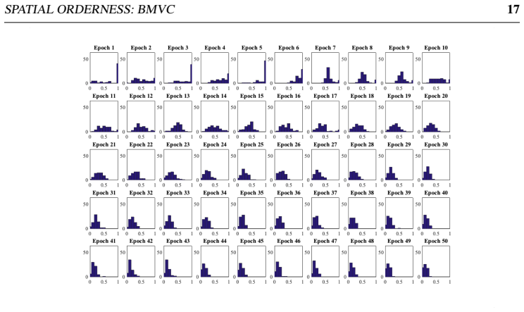
During training, feature-map spatial orderness rises across layers in a synchronized early phase, and validation accuracy only begins to improve after the deepest feature maps' orderness starts falling.
Trained kernel orderness is controlled by the input's orderness and by kernel size: smaller kernels produce more spatially ordered filters, and very large kernels behave like fully connected layers.
The correlation between the final feature map's orderness and the improvement from adding the next convolution layer implies that each convolution layer's usefulness depends on the spatial order in the feature map it receives.

Reading between the lines

Editorial extensions of the paper, not claims the author makes directly.

A direct testable extension would apply the metric to non-image data by replacing pixel neighborhoods with adjacency, for example spectrogram time-frequency bins or graph edges; the prediction is that locality-preserving architectures gain depth only when that adjacency carries order.
The early-training rise in feature-map orderness, if it is robust across architectures, could serve as a training diagnostic: validation gains should not be expected until layer-wise orderness begins to decline, and early stopping before that phase may waste the useful part of training.
The kernel-size result suggests that layer-wise kernel orderness could act as a post-hoc measure of how convolutional a layer really is, bridging the gap between architectural labels and learned behavior.
If the mechanism is right, architecture selection should become data-dependent in a quantitative way: measure the data's spatial-order profile first, then choose how many convolutional stages to stack rather than defaulting to maximum depth.

Share X Bluesky LinkedIn Reddit HN

Signed reviews

No signed human review yet.

Editorial analysis

A structured set of objections, weighed in public.

Desk editor's note, referee report, and a circularity audit.

Desk Editor's Note

read the letter

The spatial orderness metric is a simple ratio of squared intensity differences at one-hop versus two-hop lags, which is standard spatial statistics, but pointing it at CNN feature maps and kernels is new, and the block-swap experiments are a neat way to probe when depth stops paying. The three-dataset demonstration gives the empirical story some breadth.

The main observation—that adding conv layers yields diminishing or negative returns as block-swapping increases—is plausible, but the stress-test is right: block-swapping does not isolate spatial order. It also relocates class-discriminative structure, changes the boundary statistics, and makes the task objectively harder. A deeper network on a harder task can overfit and show the same curve. There is no control that raises task difficulty while preserving spatial orderness, so the headline claim is not established. The supplementary correlation in Table 1 inherits the same confound.

The feature-map dynamics (synchronized peaking then decline) are interesting descriptively, but they are not backed by error bars or repeated runs in the main text. The theory in Appendix A is the weakest part. Theorem 1's alpha is defined after the fact and can absorb any scale; the second inequality just substitutes the definition of spatial orderness, making it an identity, not a derivation. Corollaries 1.1 and 1.2 inherit the vacuity. This section should be removed or substantially rewritten, because as written it is not a theorem about CNNs—it is an algebraic restatement with free parameters.

Credit where it is due: the metric is trivial to compute and the experiments are reproducible in principle. Section 5.2 does repeat six random splits for MNIST-1000, which is more than many papers at this level, but Figure 2 lacks such statistics.

Who gets value: someone looking for a cheap diagnostic for when depth helps, or a discussion of the pitfalls of corruption-based ablation studies. It is not a paper that resolves the question, but it asks the right question.

For peer review: send it out. A serious referee should ask for the task-difficulty control and a rewritten or deleted theory section. It is a conditional accept at best, but the empirical kernel is worth discussing.

Referee Report

4 major / 4 minor

Summary. The paper introduces a multi-scale statistical metric called spatial orderness, which measures how well pixel values follow the underlying spatial grid, and uses it to investigate the behavior of CNNs. The authors block-swap images from MNIST, Fashion-MNIST, and CIFAR-10 to disrupt spatial orderness, and report that the performance improvement from adding convolutional layers shrinks and sometimes becomes negative as the amount of block-swapping increases. They also observe that feature-map spatial orderness rises then falls during training, with validation accuracy improving only after the falling phase. Finally, they present theorems (Appendix A) intended to show that kernel spatial orderness is related to input spatial orderness and that smaller kernels produce more spatially ordered kernels, with supporting experiments on MNIST-1000.

Significance. If the central finding were established, the paper would provide a useful data-centric criterion for when convolutional depth helps: the benefit of adding conv layers would depend on the presence of multi-scale spatial order in the input. The spatial orderness metric is simple and easy to compute, and the feature-map dynamics are an interesting descriptive observation that could motivate further work. However, the main empirical claim is confounded by task-difficulty changes induced by block-swapping, and the theoretical results in Appendix A are vacuous because the free constant alpha can absorb all scales and the second inequality is essentially the definition of spatial orderness. As a result, the paper's headline claims are not currently supported.

major comments (4)

[Section 4.1.2, Figure 2] The block-swapping procedure changes not only the spatial orderness of the inputs but also the difficulty of the classification task, because it moves class-discriminative image parts into atypical positions and introduces boundary discontinuities. The paper reports no control condition that increases task difficulty while leaving spatial orderness intact (e.g., label noise or a permuted-label baseline), so the diminishing and negative depth gains in Figure 2 are also consistent with a pure task-difficulty or capacity story. This confound directly affects the abstract's headline claim that convolutional depth is counterproductive for data bereft of spatial order.
[Appendix A, Theorem 1, Eq. (10)] The constant alpha = sum_n C_n^2 N_total is a free parameter that is not bounded below, and the proof only shows that the kernel difference is at most alpha times the input difference for some alpha. Since alpha can be chosen arbitrarily large after the fact, the inequality is always satisfiable and carries no falsifiable content. As a result, the stated conclusion that kernel spatial orderness is 'likely to be higher' for higher input orderness is not entailed by the theorem.
[Appendix A, Theorem 1, Eq. (11)] The second inequality of Theorem 1 is circular: it substitutes the definition of spatial orderness, so(X)_1 = E|X(a)-X(c)|^2 / E|X(a)-X(b)|^2 - 1, into the upper bound, so the claimed relationship between input orderness and kernel orderness is an identity rather than a derivation. No independent bound on the kernel's spatial orderness is obtained, and the 'prediction' is therefore not testable in the form presented.
[Section 5.2, Corollary 1.1, Figure 4(b)] The empirical claim that larger kernels yield lower kernel spatial orderness is not a valid test of the theory, because Corollary 1.1 introduces alpha(K) as an unspecified function of kernel size. Without a characterization of alpha(K), any observed trend can be absorbed into that constant, so the experiment in Figure 4(b) does not confirm the theoretical prediction. Additionally, the experiments use only 1000 MNIST examples and six random splits with no error bars shown, limiting confidence in the trend.

minor comments (4)

[Section 3, Eq. (6)] The spatial orderness metric is not restricted to [0,1]; the paper should state its range and discuss cases where the ratio E[(p-r)^2]/E[(p-q)^2] is less than 1, which would give negative values.
[Section 4.2.1] The 'synchronized peaking' of feature-map spatial orderness is reported for a single training run per dataset; adding repeated trials with error bars would strengthen this descriptive claim.
[Section 2 and Appendix A] The symbol sigma is used both for the standard deviation in the diffusion model (Eqs. 1-3) and for the noise parameters in Corollary 1.1 (Eq. 13); this overloading is confusing and should be disambiguated.
[Figure 2] The semilog plots make error-rate changes difficult to compare across datasets and conditions; consider plotting on a linear scale or reporting the actual error values with error bars.

Circularity Check

2 steps flagged · score 6.0 of 10

Theorem 1's input-to-kernel spatial-orderness link is the metric definition reinserted into a Cauchy-Schwarz bound, with a free constant making it unfalsifiable; the main depth experiment is independent but confounded.

self definitional [Supplementary Material A, Theorem 1, proof equation (11), with Eq. (6) in Section 3]
"From Theorem 1 proof: "E_{p,r}[|w(p)-w(r)|^2] ≤ α E_{a,c,n}[|Xn(a)-Xn(c)|^2] ≤ α(1+so(X)_1) E_{a,b,n}[|Xn(a)-Xn(b)|^2]"; with Eq. (6): "so(I)_1 = (E_i[(In(i)(pi)-In(i)(ri))^2] / E_i[(In(i)(pi)-In(i)(qi))^2]) - 1"."

Substituting Eq. (6) into the theorem, (1+so(X)_1)·E_{a,b}[|Xn(a)-Xn(b)|^2] = E_{a,c}[|Xn(a)-Xn(c)|^2] identically, so the second inequality is just the first inequality with c replacing b. The so(X)_1 factor is the definition of spatial orderness being inserted, not a derived relation between kernel weights and input orderness. Therefore the claimed implication 'spatial orderness of the kernels are likely to be higher when the inputs themselves have higher spatial orderness' (Section 5.1) restates the metric's definition inside a bound; no independent content about kernels is proven.
other [Supplementary Material A, Theorem 1 statement; Section 5.2 empirical validation]
"Theorem 1: "Then we must have, E_{p,q}[|w(p)-w(q)|^2] ≤ α E_{a,b,n}[|Xn(a)-Xn(b)|^2], and E_{p,r}[|w(p)-w(r)|^2] ≤ α(1+so(X)_1) E_{a,b,n}[|Xn(a)-Xn(b)|^2], for a certain non-zero valued α." Section 5.2: "We find that they conform to the predictions of our theoretical results.""

Because α is unconstrained in the statement, for any trained kernel and any input one can choose α large enough to satisfy both inequalities; the bound cannot fail. The 'validation' in Section 5.2 therefore confirms an adjustable inequality, not a quantitative prediction derived from spatial orderness. The direction of the empirical effect (e.g., smaller kernels give more ordered kernels) is not fixed by the theorem, since α(K) is also an unspecified function of K in Corollary 1.1. Thus the theoretical 'prediction' reduces to the existence of a constant, which is guaranteed by the Cauchy-Schwarz step.

full rationale

The paper's central empirical claim—that added convolutional depth yields decreasing returns when block-swapping removes high-scale spatial order (Section 4.1.2)—is an experiment with independent content; it is not derived from the spatial orderness definition by construction, and it does not depend on self-citations. Its causal interpretation is weakened by a confound: block-swapping also changes task difficulty and the image-to-label mapping, so the depth-benefit curves may reflect capacity or difficulty effects rather than a spatial-order mechanism. That is a validity concern, not circularity. The genuine circularity is in the supporting theory: Theorem 1's second inequality is the definition of so(X)_1 inserted into the first bound, and the free constant α makes the inequalities unfalsifiable, so the kernel-orderness 'predictions' validated in Section 5.2 reduce by construction. No load-bearing self-citations or imported uniqueness theorems are present. Overall, partially circular in one theoretical contribution, while the main depth experiment stands independently.

Assumptions & free parameters 4 free parameters · 4 assumptions · 0 invented entities

The metric itself has no fitted constants, but the experimental and theoretical claims rely on several unexamined modeling choices: the diffusion model, the block-swapping protocol, and a vacuous bound in the kernel theorem. The central empirical finding is conditional on these choices.

free parameters (4)

scale parameter a
Multi-scale spatial orderness is computed by averaging over a x a blocks, but the paper does not specify the values of a used for the reported scale axes; the metric's values depend on this choice (Section 3).
number of sampled triples l
The orderness estimate in Eq. (6) uses l randomly extracted pixel triples per image set; l is not specified, so the variance of the estimator is unknown (Section 3).
block-swap count Ns = 0, 10, 20, 30
The experimental conditions for spatial disruption are chosen by hand and affect the measured orderness and accuracy; there is no principled criterion for these values (Section 4.1.1).
block size k = 6, 6, 8
Chosen per dataset without justification; the choice determines which scales are disrupted (Section 4.1.1).

assumptions (4)

domain assumption Spatial data follows a Gaussian diffusion process over two-hop neighborhoods, giving E[(X(p)-X(r))^2] = 2 E[(X(p)-X(q))^2].
Used to define spatial orderness in Section 2; if real images do not follow this relation, the metric's interpretation as degree of spatial order is not established.
domain assumption Block-swapping alters spatial orderness at scales above the block size while leaving lower-scale order intact.
Section 4.1 relies on this to attribute the drop in depth benefit to loss of higher-scale order; no baseline condition isolates task difficulty.
ad hoc to paper Kernel weight updates during training are exactly Delta W = -eta(t) X rect delta, with no weight decay, momentum, or other regularizers.
Theorem 1 in Appendix A derives all bounds from this update rule; real training uses additional terms, so the bound's validity is unclear.
ad hoc to paper The undetermined constant alpha in Theorem 1 is fixed and independent of the input distribution and training dynamics.
The theorem claims existence of alpha, but alpha depends on all backprop errors and training details, so the bound does not establish the claimed monotonic relationship between input order and kernel order.

how reviews work

0 comments

Cite this review

Pith. "Pith review of Investigating Convolutional Neural Networks using Spatial Orderness." pith.science (2026). https://pith.science/paper/Y6BSUL56

@misc{pith2026190806416,
  author       = {Pith},
  title        = {Pith review of: Investigating Convolutional Neural Networks using Spatial Orderness},
  year         = {2026},
  howpublished = {\url{https://pith.science/paper/Y6BSUL56}},
  note         = {Machine review of arXiv:1908.06416}
}

read the original abstract

Convolutional Neural Networks (CNN) have been pivotal to the success of many state-of-the-art classification problems, in a wide variety of domains (for e.g. vision, speech, graphs and medical imaging). A commonality within those domains is the presence of hierarchical, spatially agglomerative local-to-global interactions within the data. For two-dimensional images, such interactions may induce an a priori relationship between the pixel data and the underlying spatial ordering of the pixels. For instance in natural images, neighboring pixels are more likely contain similar values than non-neighboring pixels which are further apart. To that end, we propose a statistical metric called spatial orderness, which quantifies the extent to which the input data (2D) obeys the underlying spatial ordering at various scales. In our experiments, we mainly find that adding convolutional layers to a CNN could be counterproductive for data bereft of spatial order at higher scales. We also observe, quite counter-intuitively, that the spatial orderness of CNN feature maps show a synchronized increase during the intial stages of training, and validation performance only improves after spatial orderness of feature maps start decreasing. Lastly, we present a theoretical analysis (and empirical validation) of the spatial orderness of network weights, where we find that using smaller kernel sizes leads to kernels of greater spatial orderness and vice-versa.

Figures

Figures reproduced from arXiv: 1908.06416 by the authors.

**Figure 2.** Semilog plots showing the test error rate of networks of different depths, trained [PITH_FULL_IMAGE:figures/full_fig_p006_2.png] view at source ↗

**Figure 3.** (a), (b) and (c) show the progression of mean spatial orderness of the feature maps [PITH_FULL_IMAGE:figures/full_fig_p007_3.png] view at source ↗

Figures from the paper (5 more)

**Figure 4.** Figure 4: (a) demonstrates that disruption of spatial orderness at the input has an immediate [PITH_FULL_IMAGE:figures/full_fig_p008_4.png]

**Figure 5.** Figure 5: A CNN with two convolutional layers of 3 [PITH_FULL_IMAGE:figures/full_fig_p014_5.png]

**Figure 6.** Figure 6: A CNN with three convolutional layers of 3 [PITH_FULL_IMAGE:figures/full_fig_p015_6.png]

**Figure 7.** Figure 7: Correlation between spatial orderness of the input data at scales (2,4 and 6), and [PITH_FULL_IMAGE:figures/full_fig_p016_7.png]

**Figure 8.** Figure 8: Shown are the histograms of the spatial orderness measures of the feature maps of [PITH_FULL_IMAGE:figures/full_fig_p017_8.png]

Discussion (0). Continue with ORCID to comment.

Reference graph

Works this paper leans on

16 extracted references · 11 canonical work pages

[1]

Scaling learning algorithms towards AI

Yoshua Bengio and Yann Lecun. Scaling learning algorithms towards AI. MIT Press, 2007

work page 2007
[2]

Representation learning: A review and new perspectives

Yoshua Bengio et al. Representation learning: A review and new perspectives. IEEE Trans. Pattern Anal. Mach. Intell., 35(8):1798–1828, August 2013. ISSN 0162-8828. doi: 10.1109/TPAMI.2013.50

doi:10.1109/tpami.2013.50 2013
[3]

Approximating CNNs with bag-of-local- features models works surprisingly well on ImageNet

Wieland Brendel and Matthias Bethge. Approximating CNNs with bag-of-local- features models works surprisingly well on ImageNet. In ICLR, 2019

work page 2019
[4]

He et al

K. He et al. Deep residual learning for image recognition. In 2016 IEEE Conf. on Computer Vision and Pattern Recognition (CVPR) , pages 770–778, June 2016. doi: 10.1109/CVPR.2016.90

doi:10.1109/cvpr.2016.90 2016
[5]

Measuring the tendency of CNNs to learn surface statis- tical regularities

Jason Jo and Yoshua Bengio. Measuring the tendency of CNNs to learn surface statis- tical regularities. ArXiv, abs/1711.11561, 2017

arXiv 2017
[6]

Generalization in deep learning

Kenji Kawaguchi et al. Generalization in deep learning. In Mathematics of Deep Learning, Cambridge University Press, to appear., 2018

work page 2018
[7]

Learning multiple layers of features from tiny images

Alex Krizhevsky. Learning multiple layers of features from tiny images. Technical Report TR-2009, University of Toronto, Toronto, 2009

work page 2009
[8]

Y . Lecun. The MNIST database of handwritten digits. http://yann.lecun.com/exdb/mnist/

work page

Show all 16 references

[9]

Understanding the effective receptive ﬁeld in deep convolutional neural networks

Wenjie Luo, Yujia Li, Raquel Urtasun, and Richard Zemel. Understanding the effective receptive ﬁeld in deep convolutional neural networks. In D. D. Lee, M. Sugiyama, U. V . Luxburg, I. Guyon, and R. Garnett, editors,Advances in Neural Information Processing Systems 29, pages 4...

2016
[10]

H. N. Mhaskar and T. Poggio. Deep vs. shallow networks: An approximation theory perspective. Analysis and Applications, 14(06):829–848, 2016

2016
[11]

Simonyan and A

K. Simonyan and A. Zisserman. Very deep convolutional networks for large-scale image recognition. In ICLR, 2015

2015
[12]

On the depth of deep neural networks: A theoretical view

Shizhao Sun et al. On the depth of deep neural networks: A theoretical view. In AAAI Conf. on Artiﬁcial Intelligence, AAAI’16, pages 2066–2072. AAAI Press, 2016. SPA TIAL ORDERNESS: BMVC 11

2016
[13]

Regularization of neural networks using dropconnect

Li Wan et al. Regularization of neural networks using dropconnect. In ICML, pages 1058–1066, 2013

2013
[14]

Fashion-MNIST: a novel image dataset for benchmarking machine learning algorithms

Han Xiao et al. Fashion-MNIST: a novel image dataset for benchmarking machine learning algorithms. ArXiv, abs/1708.07747, 2017

2017 arXiv
[15]

Zeiler and Rob Fergus

Matthew D. Zeiler and Rob Fergus. Visualizing and understanding convolutional net- works. In ECCV 2014, 2014

2014
[16]

effective

Pan Zhou and Jiashi Feng. Understanding generalization and optimization performance of deep CNNs. ICML, 2018. A Theorems Please refer to section 5 in the main paper for the implications of the theorems, and empirical validation of the theoretical results. Theorem 1. Consider a...

2018

Pith tools

Reviewed August 14, 2026 · model on record in the stance chip above.

[1] [1]

Scaling learning algorithms towards AI

Yoshua Bengio and Yann Lecun. Scaling learning algorithms towards AI. MIT Press, 2007

work page 2007

[2] [2]

Representation learning: A review and new perspectives

Yoshua Bengio et al. Representation learning: A review and new perspectives. IEEE Trans. Pattern Anal. Mach. Intell., 35(8):1798–1828, August 2013. ISSN 0162-8828. doi: 10.1109/TPAMI.2013.50

doi:10.1109/tpami.2013.50 2013

[3] [3]

Approximating CNNs with bag-of-local- features models works surprisingly well on ImageNet

Wieland Brendel and Matthias Bethge. Approximating CNNs with bag-of-local- features models works surprisingly well on ImageNet. In ICLR, 2019

work page 2019

[4] [4]

He et al

K. He et al. Deep residual learning for image recognition. In 2016 IEEE Conf. on Computer Vision and Pattern Recognition (CVPR) , pages 770–778, June 2016. doi: 10.1109/CVPR.2016.90

doi:10.1109/cvpr.2016.90 2016

[5] [5]

Measuring the tendency of CNNs to learn surface statis- tical regularities

Jason Jo and Yoshua Bengio. Measuring the tendency of CNNs to learn surface statis- tical regularities. ArXiv, abs/1711.11561, 2017

arXiv 2017

[6] [6]

Generalization in deep learning

Kenji Kawaguchi et al. Generalization in deep learning. In Mathematics of Deep Learning, Cambridge University Press, to appear., 2018

work page 2018

[7] [7]

Learning multiple layers of features from tiny images

Alex Krizhevsky. Learning multiple layers of features from tiny images. Technical Report TR-2009, University of Toronto, Toronto, 2009

work page 2009

[8] [8]

Y . Lecun. The MNIST database of handwritten digits. http://yann.lecun.com/exdb/mnist/

work page