REVIEW 3 major objections 5 minor 42 references
Modeling Time to Open of Emails with a Latent State for User Engagement Level
T0 review · 3 major / 5 minor · reviewed 2026-08-14 · deepseek-v4-flash
Pith's one-line read The paper claims that a mixture survival model predicts email open times more accurately than alternatives in a domain where most emails are never opened.
desk verdict Careful application of a known cure-mixture Cox model to email open-time data, but the headline accuracy claim is fragile: the MM advantage over linear regression on the test split is within the sampling noise the paper itself documents. read the letter →
The pith
A machine-rendered reading of the paper's core claim, the machinery that carries it, and where it could break.
The reading
What carries the argument
The machine that carries the argument is the mixture survivor function $$S_i(t|X_i)=\pi(Z_i)\,S(t|L_i=1,X_i)+(1-\pi(Z_i)),$$ where $\pi(Z_i)$ is a logistic-regression estimate of the probability that recipient $i$ belongs to the latent prone-to-open state, and $S(t|L_i=1,X_i)=S_0(t)^{\exp(\beta^T X_i)}$ is the Cox proportional-hazards survivor curve for that state. The $(1-\pi)$ term anchors non-prone recipients at survival probability 1, so each individual's predicted time-to-open is read from a low percentile of this survivor curve, the paper uses the 5th percentile, rather than the median, which is undefined when the curve flattens above 0.5. Parameters are estimated by an expectation-maximization (EM) procedure because the state indicator $L_i$ is latent. This machinery separates will-eventually-open from never-opens and fits the timing model only on the former group.
What would settle it
Re-run the comparison after extending the observation window to 30 days and re-estimating each model with a 12-hour censoring window; if the mixture model's MRAD(O) no longer beats linear regression and CoxPH, then the never-open assumption, not genuine timing accuracy, was producing the reported gain.
Extended reading notes
Core claim
On email data where roughly 8% of recipients open a message within ten days, the paper claims that a cure-mixture version of the Cox model is the right way to predict time-to-open. Each recipient has a latent indicator: those who will not open the email have survival probability 1 at every time, while those who may open follow a proportional-hazards model with a baseline hazard estimated nonparametrically, and the mixing probability is predicted by logistic regression from engagement features. On the held-out Test set, the mixture model attains a mean relative absolute deviation over opened emails of 7.381, 9.340, and 11.653 for censoring windows of 3, 6, and 12 hours, lower than linear regression (7.753, 10.194, 13.409), CoxPH with a linear relative hazard (10.009, 23.227, 29.131), and gradient-boosted Cox (13.787, 18.339, 21.080), while matching those models in area under the ROC curve. The central discovery is that explicitly modeling a subpopulation that never opens is what makes time predictions accurate when censored rows dominate.
Load-bearing premise
The load-bearing premise is that a recipient placed in the non-prone state has survival probability exactly 1 forever, while the data only observe ten days, so anyone who opens after the censoring window is treated as a never-opener; if those late openers behave differently, the model's advantage could be an artifact.
Editorial extensions
If this is right
- For marketing campaigns with open rates near 8–10%, the paper's results imply that a mixture cure model should be used instead of plain Cox regression or linear regression for open-time prediction, because its held-out mean relative absolute deviation over opened emails (MRAD(O)) is lower for every censoring window tested.
- A single survival model can provide both the probability that an email is opened and the predicted time of opening, so practitioners need not train a separate classifier and regressor, provided they accept the latent never-open state.
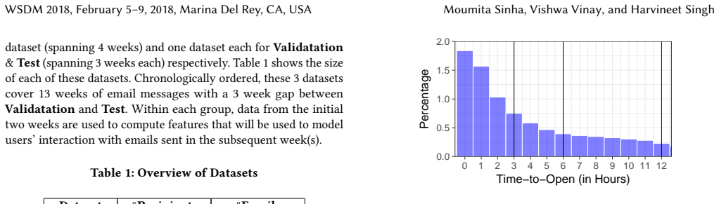
- The censoring window is a modeling choice that changes both the training data and the ranking of models: at 3 hours over half of eventual opens look censored and the mixture model's edge over linear regression is modest, while at 6 and 12 hours the gap widens.
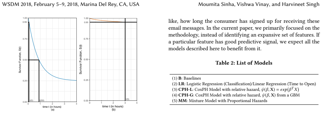
- Because the median survival time is undefined in this regime, time-to-open should be predicted from a low percentile, the 5th, of the individual survivor curve; higher percentiles saturate at the censoring window and match the baseline's error.
- Model selection should use a metric aligned with the task: tuning by AUC does not necessarily minimize MRAD, so deployments that care most about timing accuracy should validate on MRAD.
Reading between the lines
- Editorial extension: the same mixture-Cox construction should transfer to other domains with large never-event subpopulations, such as customer churn, app re-engagement, or support-ticket resolution, where censoring rates are high and a latent long-term non-event state is plausible.
- Editorial inference: because anyone who opens after the censoring window is assigned to the non-prone state, the latent states themselves depend on the chosen horizon; one could re-fit at a 12-hour window and evaluate at 3 hours to see whether the predicted early-window distribution changes.
- Beyond the paper: the reported advantage is aggregate; a follow-up could examine whether the mixture model's gain concentrates in recipients with high historical engagement or in cold recipients, which would identify the segment driving the improvement.
Signed reviews
Editorial analysis
A structured set of objections, weighed in public.
Referee Report
Summary. The paper addresses prediction of whether and when a recipient opens a marketing email. It casts the problem in a survival-analysis framework with censoring windows of 3, 6, and 12 hours and compares (i) simple baselines, (ii) logistic/linear regression, (iii) Cox proportional hazards with a linear relative hazard, (iv) Cox with a gradient-boosted hazard, and (v) a mixture cure-style Cox model in which a logistic regression assigns a latent probability of being 'prone to open' and a Cox model governs open times for the prone group. Using a large proprietary email dataset split into Training, Validation, and Test sets, the paper reports AUC and mean relative absolute deviation, checks proportional-hazards assumptions with Schoenfeld residuals, examines the effect of the survival percentile p used for time prediction, runs a bootstrap stability experiment, and evaluates out-of-time on Test. The headline claim is that the mixture model achieves the best time-to-open accuracy, especially at the 3-hour censoring window.
Significance. If the empirical claim were established at the reported precision, the paper would make a useful applied contribution: it demonstrates a principled survival-analysis treatment of 'never-event' recipients in email marketing, where the open rate is low, and it checks model assumptions carefully. The evaluation is structured, with separate train/validation/test sets, bootstrap stability results, and an out-of-time holdout, which is a strength. The assumption checks (Schoenfeld residuals and group survival curves) are appropriate for the Cox framework. However, the central 'best accuracy' claim is not supported at the required precision: the reported Test advantage is smaller than the model's own bootstrap variability, and the advantage disappears at the next percentile. Because these concerns are about evidence rather than about the model's mathematical viability, they can be addressed by additional analysis.
major comments (3)
- [§4.5, Table 6; §4.4, Table 5] The central claim that MM is the most accurate model for time-to-open rests on a single Test split. At C=3 hours, Table 6 reports MRAD(O)=7.381 for MM versus 7.753 for LR, a difference of 0.372. Table 5 shows that on the Validation set the bootstrap standard deviation of MM's MRAD(O) is 1.854 and its mean is 9.277, whereas LR has mean 8.215 with SD 0.036; on Validation, LR is actually better. The paper itself states in §4.4 that confidence intervals would be 'required if we were to reliably order the different models.' No such interval is supplied for the Test comparison, so the ordering MM<LR at C=3h is not established.
- [§4.3, Table 4] The reported time-prediction advantage of MM is confined to a single percentile choice. For C=3 hours, MM's MRAD(O) is 9.499 at p=5 but jumps to 26.641 at p=10, exactly the value of the constant censoring-window baseline B in Table 3. The same pattern holds at C=6 and 12 hours, where p>=25 (or p>=10) reproduces the baseline. Since §4.5 selects p as the value with lowest validation MRAD, the Test result depends on a one-point selection in the percentile grid. The paper should report Test MRAD(O) for all p values (at least p=5 and p=10) and account for the selection, or otherwise show that the comparison is not an artifact of this choice.
- [§2.2, Eq. (9); §3.1] The mixture model's latent state is defined as 'prone to the event' but is estimated from data censored at 3, 6, or 12 hours, while opens are monitored for 10 days. With C=3 hours, roughly 57% of eventual opens are censored (§3.1). Under Eq. (9), censored individuals can be assigned to the non-prone state with survival probability 1, so L_i conflates 'will never open' with 'did not open within the window.' This makes the engagement interpretation and the predicted times depend on the chosen censoring horizon. The paper should assess sensitivity of the MM advantage to this conflation, for example by evaluating a model that allows late opens or by reporting the proportion of censored observations assigned to L=0.
minor comments (5)
- [§2.2, Eq. (10)] The likelihood expression is not written in a standard form: the hazard term h(t_i | L_i, X_i) appears inside an exponent indexed by the latent state L_i, even though L_i is unobserved. Please clarify the exact EM objective used for estimation.
- [§3.1.1] Using the same symbol LR for both logistic and linear regression, with only a footnote to disambiguate, makes Tables 3, 5, and 6 hard to read; consider separate names or explicit column labels.
- [§4.4] The phrase '10 bootrapped samples' should read '10 bootstrapped samples'; with only 10 bootstrap replicates, the standard-deviation estimates themselves have high variability, so the reported SDs should be interpreted cautiously.
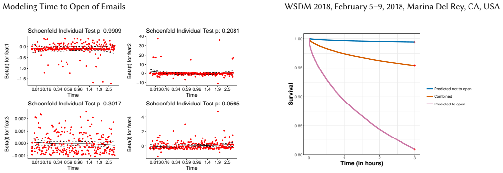
- [§3.2, Figure 3] Only CPH-L Schoenfeld residuals are shown, although the text states that the procedure can be applied to GBM and MM; either show the analogous plots or state explicitly that the displayed checks are for the linear Cox model.
- [§4.3, Table 4] Table 4 does not include the LR baseline, which makes it harder to compare the p-sensitivity of the winning model with the linear-regression baseline; adding LR would strengthen the analysis.
Circularity Check
No circularity: MM is fitted on training/validation data and evaluated on held-out Test data; no predicted quantity is a fitted parameter renamed, and no load-bearing self-citation appears.
full rationale
The derivation chain is self-contained and empirical, not definitional. The CoxPH model (Eqs. 4-6) is the standard proportional-hazards partial-likelihood model, and the mixture model (Eqs. 7-10) is the standard mixture-cure formulation cited to Farewell (1982) and Branders et al. (2015), both external sources. The latent state L_i is estimated by EM from the training data, not defined in terms of the test quantity being predicted. Time-to-open predictions are obtained from each individual's fitted survival curve by inverting S_i(t) at a percentile p (Section 3.3), with p selected on the Validation set (Section 4.5); the headline MRAD(O) numbers in Table 6 are then computed on the held-out Test set. No fitted parameter is algebraically identified with the reported metric, and no self-citation is used as load-bearing support. The mixture model's cure assumption (non-prone recipients have S(t)=1) is a modeling choice, and the paper explicitly acknowledges the possibility that it may not match all late openers; this is a correctness/misspecification concern, not circularity. The paper also candidly notes in Section 4.4 that bootstrap confidence intervals "would be required if we were to reliably order the different models," which flags statistical reliability of the model ordering but does not indicate that any prediction reduces to its input by construction. Overall, no circular step is present; the score is 0.
Assumptions & free parameters
free parameters (4)
- Survival percentile p for time prediction =
5 (selected on Validation for MM)
- Elastic Net hyperparameters lambda and alpha =
not reported (selected via Validation)
- GBM hyperparameters =
not reported (selected via Validation)
- Censoring window C_i =
3, 6, 12 hours (evaluated separately)
assumptions (5)
- domain assumption Non-informative censoring: the censoring time C is independent of the potential time-to-open.
- domain assumption Cure fraction: the latent non-prone group has survival probability 1 for all t (they will never open).
- domain assumption Proportional hazards within the prone group and for CoxPH models.
- domain assumption Features are time-invariant covariates (no time-dependent features).
- domain assumption Logistic regression correctly specifies the probability of being in the prone group pi(Z_i).
invented entities (1)
-
Latent engagement state L_i
Cite this review
Pith. "Pith review of Modeling Time to Open of Emails with a Latent State for User Engagement Level." pith.science (2026). https://pith.science/paper/IFRFOQG6
@misc{pith2026190806512,
  author       = {Pith},
  title        = {Pith review of: Modeling Time to Open of Emails with a Latent State for User Engagement Level},
  year         = {2026},
  howpublished = {\url{https://pith.science/paper/IFRFOQG6}},
  note         = {Machine review of arXiv:1908.06512}
}
read the original abstract
Email messages have been an important mode of communication, not only for work, but also for social interactions and marketing. When messages have time sensitive information, it becomes relevant for the sender to know what is the expected time within which the email will be read by the recipient. In this paper we use a survival analysis framework to predict the time to open an email once it has been received. We use the Cox Proportional Hazards (CoxPH) model that offers a way to combine various features that might affect the event of opening an email. As an extension, we also apply a mixture model (MM) approach to CoxPH that distinguishes between recipients, based on a latent state of how prone to opening the messages each individual is. We compare our approach with standard classification and regression models. While the classification model provides predictions on the likelihood of an email being opened, the regression model provides prediction of the real-valued time to open. The use of survival analysis based methods allows us to jointly model both the open event as well as the time-to-open. We experimented on a large real-world dataset of marketing emails sent in a 3-month time duration. The mixture model achieves the best accuracy on our data where a high proportion of email messages go unopened.
Figures

Figures from the paper (1 more)
Reference graph
Works this paper leans on
-
[1]
Sattar Ameri, Mahtab J. Fard, Ratna B. Chinnam, and Chandan K. Reddy. 2016. Survival Analysis Based Framework for Early Prediction of Student Dropouts. In Proceedings of the 25th ACM International on Conference on Information and Knowledge Management (CIKM ’16) . ACM, New York, NY, USA, 903–912. https: //doi.org/10.1145/2983323.2983351
arXiv 2016
-
[2]
Nicola Barbieri, Fabrizio Silvestri, and Mounia Lalmas. 2016. Improving post-click user engagement on native ads via survival analysis. In Proceedings of the 25th International Conference on World Wide Web . International World Wide Web Conferences Steering Committee, 761–770
work page 2016
-
[3]
André Bonfrer and Xavier Drèze. 2009. Real-time evaluation of e-mail campaign performance. Marketing Science 28, 2 (2009), 251–263
work page 2009
-
[4]
Samuel Branders, Roberto D’Ambrosio, and Pierre Dupont. 2015. A mixture Cox-Logistic model for feature selection from survival and classification data. arXiv preprint arXiv:1502.01493 (2015)
work page Pith review arXiv 2015
-
[5]
Harry B Burke, Philip H Goodman, David B Rosen, Donald E Henson, John N Weinstein, Frank E Harrell, Jeffrey R Marks, David P Winchester, and David G Bostwick. 1997. Artificial neural networks improve the accuracy of cancer survival prediction. Cancer 79, 4 (1997), 857–862
work page 1997
-
[6]
D Chaffey. 2009. Mint.com used StrongMail Influencer to create this viral program. http://www.strongmail.com/pdf/sm_casestudy_mint.pdf. (2009)
work page 2009
-
[7]
Sunandan Chakraborty, Filip Radlinski, Milad Shokouhi, and Paul Baecke. 2014. On Correlation of Absence Time and Search Effectiveness. In Proceedings of the 37th International ACM SIGIR Conference on Research & Development in Information Retrieval (SIGIR ’14) . ACM, New York, NY, USA, 1163–1166. https: //doi.org/10.1145/2600428.2609535
arXiv 2014
-
[8]
Anurat Chapanond, Mukkai S Krishnamoorthy, and Bülent Yener. 2005. Graph theoretic and spectral analysis of Enron email data. Computational & Mathemat- ical Organization Theory 11, 3 (2005), 265–281
work page 2005
Show all 42 references
-
[9]
Gordon V. Cormack. 2008. Email Spam Filtering: A Systematic Review. In Foun- dations and Trends in Information Retrieval , Vol. 1
2008
-
[10]
DR Cox. 1972. Regression models and life tables. Journal of the Royal Statistical Society 34 (1972), 187–220
1972
-
[11]
Laura Dabbish, Gina Venolia, and JJ Cadiz. 2003. Marked for Deletion: An Analysis of Email Data. In CHI ’03 Extended Abstracts on Human Factors in Computing Systems (CHI EA ’03) . ACM, New York, NY, USA, 924–925. https: //doi.org/10.1145/765891.766073
2003
-
[12]
Vachik S Dave, Mohammad Al Hasan, and Chandan K Reddy. 2017. How Fast Will You Get a Response? Predicting Interval Time for Reciprocal Link Creation.. In ICWSM. 508–511
2017
-
[13]
Dursun Delen, Glenn Walker, and Amit Kadam. 2005. Predicting breast cancer survivability: a comparison of three data mining methods. Artificial intelligence in medicine 34, 2 (2005), 113–127
2005
-
[14]
Dotan Di Castro, Zohar Karnin, Liane Lewin-Eytan, and Yoelle Maarek. 2016. You’ve Got Mail, and Here is What You Could Do With It!: Analyzing and Pre- dicting Actions on Email Messages. In Proceedings of the Ninth ACM International Conference on Web Search and Data Mining (WSD...
2016
-
[15]
Tim Drye, Graham Wetherill, and Alison Pinnock. 2001. When are customers in the market? Applying survival analysis to marketing challenges. Journal of Targeting, Measurement and Analysis for Marketing 10, 2 (2001), 179–188
2001
-
[16]
Nicolas Ducheneaut and Victoria Bellotti. 2001. E-mail as habitat: an exploration of embedded personal information management. interactions 8, 5 (2001), 30–38
2001
-
[17]
Miles Efron. 2012. Query-specific recency ranking: Survival analysis for improved microblog retrieval. In Proceedings of the TAIA-12 Workshop associated to SIGIR-12. Citeseer
2012
-
[18]
Vern T Farewell. 1982. The use of mixture models for the analysis of survival data with long-term survivors. Biometrics (1982), 1041–1046
1982
-
[19]
Patricia M Grambsch and Terry M Therneau. 1994. Proportional hazards tests and diagnostics based on weighted residuals. Biometrika (1994), 515–526
1994
-
[20]
Eric Horvitz, Andy Jacobs, and David Hovel. 1999. Attention-sensitive Alerting. In Proceedings of the Fifteenth Conference on Uncertainty in Artificial Intelligence (UAI’99). Morgan Kaufmann Publishers Inc., San Francisco, CA, USA, 305–313. http://dl.acm.org/citation.cfm?id=20...
1999
-
[21]
Anjuli Kannan, Karol Kurach, Sujith Ravi, Tobias Kaufmann, Andrew Tomkins, Balint Miklos, Greg Corrado, László Lukács, Marina Ganea, Peter Young, and Vivek Ramavajjala. 2016. Smart Reply: Automated Response Suggestion for Email. CoRR abs/1606.04870 (2016). http://arxiv.org/abs...
2016 arXiv
-
[22]
Edward L Kaplan and Paul Meier. 1958. Nonparametric estimation from incom- plete observations. Journal of the American statistical association 53, 282 (1958), 457–481
1958
-
[23]
Thomas Karagiannis and Milan Vojnovic. 2009. Behavioral Profiles for Advanced Email Features. In Proceedings of the 18th International Conference on World Wide Web (WWW ’09). ACM, New York, NY, USA, 711–720. https://doi.org/10.1145/ 1526709.1526805
2009
-
[24]
Bryan Klimt and Yiming Yang. 2004. The Enron Corpus: A New Dataset for Email Classification Research. Springer Berlin Heidelberg, Berlin, Heidelberg, 217–226. https://doi.org/10.1007/978-3-540-30115-8_22
2004 doi
-
[25]
Kumar, Xi (Alan) Zhang, and Anita Luo
V. Kumar, Xi (Alan) Zhang, and Anita Luo. 2014. Modeling Customer Opt- In and Opt-Out in a Permission-Based Marketing Context. Journal of Mar- keting Research 51, 4 (2014), 403–419. https://doi.org/10.1509/jmr.13.0169 arXiv:http://dx.doi.org/10.1509/jmr.13.0169
2014 doi
-
[26]
Carvalho, and Emine Yilmaz
Matthew Lease, Vitor R. Carvalho, and Emine Yilmaz. 2011. Crowdsourcing for Search and Data Mining. SIGIR Forum 45, 1 (May 2011), 18–24. https://doi.org/ 10.1145/1988852.1988856
2011
-
[27]
Jeong-Yoon Lee, Hang Zhang, and Valery A Petrushin. 2012. Sur- vival Analysis for Marketing. https://pdfs.semanticscholar.org/2360/ bb9ea10622c8c21595ade8f43cc237aac230.pdf. (2012). [Online; accessed 15-March-2017]
2012
-
[28]
Yan Li, Jie Wang, Jieping Ye, and Chandan K Reddy. 2016. A multi-task learning formulation for survival analysis. In Proceedings of the 22nd ACM SIGKDD Inter- national Conference on Knowledge Discovery and Data Mining . ACM, 1715–1724
2016
-
[29]
DY Lin. 2007. On the Breslow estimator. Lifetime Data Analysis 13, 4 (2007), 471–480
2007
-
[30]
Junxiang Lu and O Park. 2003. Modeling customer lifetime value using survival analysisâĂŤan application in the telecommunications industry. Data Mining Techniques (2003), 120–128
2003
-
[31]
Dumais, Nick Craswell, Dan Liebling, and Qingyao Ai
Kanika Narang, Susan T. Dumais, Nick Craswell, Dan Liebling, and Qingyao Ai
-
[32]
Rajesh Ranganath, Adler Perotte, Noémie Elhadad, and David Blei. 2016. Deep Survival Analysis. In Proceedings of the 1st Machine Learning for Healthcare Conference. 101–114
2016
-
[33]
Greg Ridgeway. 1999. The State of Boosting. (1999)
1999
-
[34]
G Tsirulnik. 2011. British Airways mobile email campaign garners 250K app down- loads. http://www.mobilemarketer.com/ex/mobilemarketer/cms/news/email/ 9056.html. (2011)
2011
-
[35]
Shar VanBoskirk, CS Overby, and S Takvorian. 2011. US interactive marketing forecast 2011 to 2016, Forrester Research. (2011)
2011
-
[36]
Jian Wang and Yi Zhang. 2013. Opportunity model for e-commerce recommenda- tion: right product; right time. In Proceedings of the 36th international ACM SIGIR conference on Research and development in information retrieval . ACM, 303–312
2013
-
[37]
Ping Wang, Yan Li, and Chandan K Reddy. 2017. Machine Learning for Survival Analysis: A Survey. Comput. Surveys (2017)
2017
-
[38]
D Wells. 2016. Email marketing statistics 2017. http://www. smartinsights.com/email-marketing/email-communications-strategy/ statistics-sources-for-email-marketing/. (2016)
2016
-
[39]
Steve Whittaker and Candace Sidner. 1996. Email overload: exploring personal information management of email. In Proceedings of the SIGCHI conference on Human factors in computing systems . ACM, 276–283
1996
-
[40]
Liu Yang, Susan Dumais, Paul Bennett, and Ahmed Hassan Awadallah. 2017. Characterizing and Predicting Enterprise Email Reply Behavior. In Proceedings of the 40th Annual International ACM SIGIR Conference on Research and Development in Information Retrieval (SIGIR 2017) . ACM
2017
-
[41]
Hui Zou and Trevor Hastie. 2005. Regularization and variable selection via the elastic net. Journal of the Royal Statistical Society: Series B (Statistical Methodology) 67, 2 (2005), 301–320
2005
-
[2017]
In Proceedings of the 2017 Conference on Conference Human Information Interaction and Retrieval (CHIIR ’17)
Large-Scale Analysis of Email Search and Organizational Strategies. In Proceedings of the 2017 Conference on Conference Human Information Interaction and Retrieval (CHIIR ’17) . ACM, New York, NY, USA, 215–223. https://doi.org/10. 1145/3020165.3020175
2017
Reviewed August 14, 2026 · model on record in the stance chip above.
Discussion (0). Continue with ORCID to comment.