REVIEW 4 major objections 4 minor 38 references
Quantum Expectation-Maximization Algorithm
T0 review · 4 major / 4 minor · reviewed 2026-08-14 · deepseek-v4-flash
Pith's one-line read A quantum EM algorithm estimates Gaussian mixture parameters with per-iteration cost growing polylogarithmically in the number of data points.
desk verdict The q-EM paper is built on a wrong distance—using Σ instead of Σ^{-1}—so the claimed exponential speedup over EM is unsupported as written. read the letter →
The pith
A machine-rendered reading of the paper's core claim, the machinery that carries it, and where it could break.
The reading
What carries the argument
The load-bearing object is the δ-EM algorithm, a randomized, noise-tolerant rewrite of EM. Its E step assigns each point a label sampled uniformly from all clusters whose square GMM distance $d^k_G(y_i)=(y_i-\mu_k)^\top \Sigma_k (y_i-\mu_k)+\ln|\Sigma_k|-2\ln(K\pi_k)$ is within $\delta$ of the best cluster, and it discards points whose best cluster lacks a $2\delta$ margin; its M step adds small Gaussian noise to the estimated parameters. On top of δ-EM, the q-EM algorithm layers the quantum k-means toolbox: amplitude estimation and median evaluation to compute the distances, a quantum argmin for label assignment, QRAM-stored data matrices $V_1$ and $V_2$ to form mean and covariance states via quantum linear algebra, and quantum vector state tomography to output classical parameters. The square GMM distance is the piece that generalizes the Euclidean distance of quantum k-means to weights and covariances, letting the same quantum machinery handle soft clustering.
What would settle it
Take a synthetic Gaussian mixture whose components are close enough that a large fraction of points have square GMM distances within $2\delta$ of two clusters, run δ-EM with the paper's $\delta$, and compare the estimated means, covariances, and weights with EM's: if the parameter bias exceeds the paper's error budgets, or if the discarded-point fraction drops cluster sizes below the assumed $\Omega(N/K)$, the equivalence premise is falsified.
Extended reading notes
Core claim
The central claim is that the q-EM algorithm realizes a quantum speedup of the δ-EM algorithm: for each iteration, the runtime is polylogarithmic in the number of data points $N$, with the explicit bound in Eq. (34) depending on the number of clusters $K$, the dimension $d$, condition numbers and norms of the data matrices, and the error parameters $\epsilon_1$, $\epsilon^\mu_3$, $\epsilon^\mu_4$, $\epsilon^\Sigma_3$, $\epsilon^\Sigma_4$, $\epsilon^\pi_4$. If correct, this is an exponential improvement over classical EM, whose E step already requires touching all $N$ points to compute responsibilities. The speedup is achieved by replacing the classical E step with a quantum computation of the square GMM distance, followed by an argmin assignment, and by generating mean and covariance quantum states through quantum linear algebra with QRAM data structures; classical parameter estimates are recovered by quantum vector state tomography. The paper is explicit that the proved speedup applies to δ-EM rather than to EM itself, and it offers numerical evidence, not an analytical bound, for the equivalence of δ-EM and EM at small δ.
Load-bearing premise
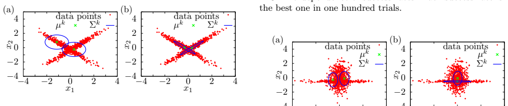
The argument assumes that the randomized δ-EM algorithm, which rounds responsibilities and discards close-to-tie points, estimates essentially the same parameters as the true EM algorithm when δ is small; the paper supports this only with two synthetic examples, not with an analytical error bound.
Editorial extensions
If this is right
- If the central claim is right, each EM-style update costs polylogarithmically in $N$ rather than a cost that scales at least linearly with $N$, so the $N$-dependence of one iteration is exponentially improved.
- The quantum algorithm outputs classical estimates of $\pi$, $\mu$, and $\Sigma$ at the end of each iteration, so it can serve as a parameter-estimation subroutine inside existing EM workflows.
- The randomized δ-EM variant inherits tolerance to quantum measurement noise and, at small $\delta$, reproduces EM's solutions on the paper's synthetic benchmarks.
- Because q-EM reduces to quantum k-means when all weights are equal and all covariances are the identity, the Gaussian-mixture result strictly generalizes the quantum k-means speedup.
- The same distance-replacement strategy is stated by the authors to extend to mixture models beyond Gaussians.
Reading between the lines
- An inference the paper does not draw: the exponential gain is per iteration, not per full run; if the number of iterations to convergence grows with $N$, the total speedup could shrink, so an end-to-end comparison needs measured iteration counts on realistic data sets.
- The equivalence of δ-EM and EM likely requires a separation condition: clusters whose square GMM distances differ by more than $2\delta$ for most points. A testable consequence is that success rates on overlapping clusters should drop as overlap increases, mirroring the $\delta$-dependence in the paper's simulations.
- A practical extension would be to use the q-EM distance estimates as a warm start or inside variational Bayes inference, whose parameter re-estimation step has the same weighted-average form as EM.
- Because the stated runtime depends on condition numbers $\kappa(V_1)$, $\kappa(V_2)$ and norms $\eta_\mu$, $\eta_\Sigma$, the speedup is only realized for well-conditioned data; a scaling test on ill-conditioned synthetic mixtures would show where the advantage disappears.
Signed reviews
Editorial analysis
A structured set of objections, weighed in public.
Referee Report
Summary. The paper proposes a quantum expectation-maximization (q-EM) algorithm for Gaussian mixture models (GMMs), following the template of the q-means algorithm of Kerenidis et al. It first introduces a randomized classical variant, the δ-EM algorithm, which replaces soft responsibilities with approximate hard assignments within a tolerance δ and adds noise in the M-step. The quantum algorithm computes a square GMM distance, assigns labels via a minimum-finding circuit, prepares quantum states for the means and covariance matrices using QRAM and quantum linear algebra, and obtains classical estimates by tomography. The main claimed result is that each iteration of q-EM runs in time polylogarithmic in the number of data points N, giving an exponential speedup over classical EM. The classical δ-EM algorithm is tested on two synthetic two-Gaussian examples, where it is reported to perform similarly to EM and better than (δ-)k-means.
Significance. If the claimed speedup were established, this work would be a meaningful step toward quantum algorithms for a broader class of clustering models than k-means. The paper honestly builds on the existing q-means framework, provides a concrete runtime expression, and includes a numerical study of the classical δ-EM variant. However, the central claim -- that q-EM is an exponentially faster EM algorithm -- is not established as written. The distance used in the algorithm is not the GMM likelihood distance, the equivalence between δ-EM and EM is only numerically illustrated, and there is an internal inconsistency in the runtime derivation. These issues are load-bearing, so the paper requires substantial revision before its central claim can be accepted.
major comments (4)
- [Section II B, Eq. (6)]
- [Section V]
- [Section III C and III E]
- [Section IV C, Eq. (34) vs Eq. (53)]
minor comments (4)
- [Section III D, Eq. (31)]
- [Section V]
- [References]
- [Section V, Figs. 1 and 2]
Circularity Check
No circularity found; runtime claim is a complexity derivation from external quantum subroutines, and δ-EM equivalence is numerically supported rather than constructionally forced.
full rationale
The paper's central runtime claim (Eq. 34) is derived from standard quantum subroutines — QRAM, amplitude estimation, median evaluation, and quantum linear algebra — cited from external work (Refs. [7, 11, 18, 20, 21]) and does not use the target speedup as an input. The δ-EM algorithm is defined in Section II B as a modified E step with a δ-ball label set and noise injection in the M step; q-EM (Algorithm 2) implements this modified algorithm, not EM as such. The paper states in Section V that the purpose is 'to see that the EM and δ-EM algorithms are equivalent when δ is sufficiently small,' but this equivalence is supported only by two synthetic numerical examples and is not given an analytical bound. That is an evidentiary gap, and the definition of d_G in Eq. (6) with Σ_k rather than Σ_k^{-1} raises a correctness concern, but neither constitutes circularity: the simulation results are not used as fitted inputs to the runtime analysis, and the speedup is not forced by an equation-level identity. Self-citations in the introduction (Refs. [13–16]) are contextual and not load-bearing for the quantum speedup claim. No fitted parameter is renamed as a prediction, no uniqueness theorem is imported from the authors' own prior work, and the derivation does not reduce to its own inputs. Therefore, no circular step is present.
Assumptions & free parameters
free parameters (2)
- δ =
0.2 (Section V)
- Noise variances in M step =
0.01 for π and μ, 0.001 for Σ (footnote [24])
assumptions (4)
- domain assumption QRAM data structure supports O(log^2 N) queries and updates
- domain assumption All cluster sizes are Ω(N/K)
- standard math Quantum linear algebra subroutines (Theorem 1, Appendix B4) are correct
- standard math Amplitude estimation and median evaluation work as stated
Cite this review
Pith. "Pith review of Quantum Expectation-Maximization Algorithm." pith.science (2026). https://pith.science/paper/RHPI6G5X
@misc{pith2026190806655,
  author       = {Pith},
  title        = {Pith review of: Quantum Expectation-Maximization Algorithm},
  year         = {2026},
  howpublished = {\url{https://pith.science/paper/RHPI6G5X}},
  note         = {Machine review of arXiv:1908.06655}
}
read the original abstract
Clustering algorithms are a cornerstone of machine learning applications. Recently, a quantum algorithm for clustering based on the k-means algorithm has been proposed by Kerenidis, Landman, Luongo and Prakash. Based on their work, we propose a quantum expectation-maximization (EM) algorithm for Gaussian mixture models (GMMs). The robustness and quantum speedup of the algorithm is demonstrated. We also show numerically the advantage of GMM over k-means for non-trivial cluster data.
Figures


Reference graph
Works this paper leans on
-
[1]
Amplitude estimation Here we sumarize the amplitude estimation algorithm that was proposed in Ref. [18]. Assume that we have UA given by UA :|0⟩↦→ √p|tari,k, 1⟩ + √ 1−p ⏐⏐gari,k, 0 ⟩ . (B1) Then, there exists an amplitude estimation algorithm that outputs ˜p such that ‖˜p−p‖≤ 2π √ p(1−p) Pae + ( π Pae )2 , (B2) with probability at least 8 /π2. The algorit...
-
[2]
(31) The associated error is ϵΣ 2
Similarly, we compute a state involving information on Σk by using quantum linear al- gebra [20, 21]: |vec[Σk t+1] +µk t+1⊗µk t+1⟩ =V2|χk t⟩. (31) The associated error is ϵΣ 2 . Note that ϵµ 2 and ϵΣ 2 appear only in logarithms; thus, we do not explicitly consider them. We finally deal with {πk}K k=1; it is relatively easy to compute the weights of the GMM...
-
[3]
To this end, we exploit the quantum random access memory (QRAM) introduced in Refs
Quantum random access memory In the q-means and q-EM algorithm, it is crucial to prepare data as a quantum state efficiently. To this end, we exploit the quantum random access memory (QRAM) introduced in Refs. [30, 31]. Here, the authors consider a device that performs the operation ∑ j ψj|j⟩a QRAM → ∑ j ψj|j⟩a|Dj⟩d. (B5) We follow the application of the QR...
-
[4]
(38) We estimate {πk}K k=1 via the distribution of labels in quantum vector state tomography. C. Runtime In the following, Eq. (34), i.e the runtime of each iter- ation of the q-EM algorithm is derived using Hoeffding’s inequality The required number of quantum vector state tomography of K mean vectors is given as follows [11]: ˜O (Kd lnK lnd (ϵµ 4)2 ) . (...
work page 2000
-
[5]
Median evaluation The time complexity of the mode evaluation algorithm is given in Lemma 8 of Ref. [7]. Let us summarize the main idea of this Lemma. Let U be a unitary operation given by U : ⏐⏐0⊗n⟩ ↦→√a|x, 1⟩ + √ 1−a|gar, 0⟩, (B3) for 1/2<a ≤ 1 in time T . Then there exists a quantum algorithm that produces a state |Φ⟩ such that ‖| Φi,k⟩−| 0⟩⊗nL|x⟩‖ 2≤ √...
-
[6]
P. Rebentrost, M. Mohseni, and S. Lloyd, Phys. Rev. Lett. 113, 130503 (2014)
work page 2014
-
[7]
LetM∈ Rd×d that satisfies‖M‖2 = 1 and x∈ Rd
Quantum linear algebra Some useful subroutines that are used in q-means and q-EM are given as follows: Theorem 1. LetM∈ Rd×d that satisfies‖M‖2 = 1 and x∈ Rd. If M is stored in QRAM and the time to prepare |x⟩ isTx, then there exist quantum algorithms that return • a state |z⟩ such that ‖|z⟩−| Mx⟩‖ ≤ϵ in time ˜O ( (κ(M)µ(M) +Txκ(M)) ln(ϵ−1) ) , • a state |...
-
[8]
P. W. Shor, SIAM review 41, 303 (1999)
1999
Show all 38 references
-
[9]
Quantum computation and quantum information,
M. A. Nielsen and I. Chuang, “Quantum computation and quantum information,” (2002)
2002
-
[10]
Biamonte, P
J. Biamonte, P. Wittek, N. Pancotti, P. Rebentrost, N. Wiebe, and S. Lloyd, Nature 549, 195 (2017)
2017
-
[11]
(18), we get |Φi,k⟩ such that ‖| Φi,k⟩−| 0⟩⊗L|˜pi,k⟩‖ 2≤ √ 2∆
to Eq. (18), we get |Φi,k⟩ such that ‖| Φi,k⟩−| 0⟩⊗L|˜pi,k⟩‖ 2≤ √ 2∆. (19) The last step is to estimate the square GMM distance of unnormalized vectors ‖yi‖ and ‖µk‖ and to multi- ply the norms of them and adding ln πk. A transla- tion operator ˆT (r′) can conduct the adding o...
- [12]
-
[13]
Schuld, I
M. Schuld, I. Sinayskiy, and F. Petruccione, Contempo- rary Physics 56, 172 (2015)
2015
- [14]
-
[15]
Dunjko, J
V. Dunjko, J. M. Taylor, and H. J. Briegel, Physical review letters 117, 130501 (2016)
2016
-
[16]
Pattern recognition and machine learning (information science and statistics), 1st edn. 2006. corr. 2nd printing edn,
C. Bishop, “Pattern recognition and machine learning (information science and statistics), 1st edn. 2006. corr. 2nd printing edn,” (2007)
2007
-
[17]
K. P. Murphy, Machine learning: a probabilistic perspec- tive (MIT press, 2012)
2012
-
[18]
Kerenidis, J
I. Kerenidis, J. Landman, A. Luongo, and A. Prakash, arXiv preprint arXiv:1812.03584 (2018)
2018 arXiv
-
[19]
A. P. Dempster, N. M. Laird, and D. B. Rubin, Journal of the Royal Statistical Society, Series B 39, 1 (1977)
1977
-
[20]
Miyahara and K
H. Miyahara and K. Tsumura, in American Control Con- ference (ACC), 2016 (2016)
2016
-
[21]
Miyahara, K
H. Miyahara, K. Tsumura, and Y. Sughiyama, in Deci- sion and Control (CDC), 2016 IEEE 55th Conference on (IEEE, 2016) pp. 4674–4679
2016
-
[22]
Miyahara, K
H. Miyahara, K. Tsumura, and Y. Sughiyama, Journal of Statistical Mechanics: Theory and Experiment 2017, 10 113404 (2017)
2017
-
[23]
Miyahara and Y
H. Miyahara and Y. Sughiyama, Physical Review A 98, 022330 (2018)
2018
-
[24]
Kerenidis, A
I. Kerenidis, A. Luong, and A. Prakash, (Private com- munication) (2019)
2019
-
[25]
Brassard, P
G. Brassard, P. Hoyer, M. Mosca, and A. Tapp, Con- temporary Mathematics 305, 53 (2002)
2002
-
[26]
[7], and it is called median evaluation in Ref
This algorithm has no specific name in Ref. [7], and it is called median evaluation in Ref. [11]. But this algorithm realize majority voting; so we call it mode evaluation
-
[27]
Chakraborty, A
S. Chakraborty, A. Gily´ en, and S. Jeffery, arXiv preprint arXiv:1804.01973 (2018)
2018 arXiv
- [28]
-
[29]
Hoeffding, in The Collected Works of Wassily Hoeffd- ing (Springer, 1994) pp
W. Hoeffding, in The Collected Works of Wassily Hoeffd- ing (Springer, 1994) pp. 409–426
1994
-
[30]
Cornell and S
D. Cornell and S. Sastry, (2015)
2015
-
[31]
In the the δ-k-means algorithm, we added Gaussian noise whose mean is 0 and variance is 0.01 to each element of all the centroids. In the M step of the δ-EM algorithm, we added Gaussian noise whose mean is 0 and variance is 0.01 to πk and each element of µk, and add Gaus- sian...
-
[32]
In Fig. 3, we draw the blue ellipses by moving θ (0≤θ< 2π) in f(θ) := µk + √ σk 1ek 1 cos(θ) + √ σk 2ek 2 sinθ where σk 1 and σk 2 are the eigenvalues of Σ k, and ek 1 and ek 2 are the corresponding eigenvectors of Σ k, respectively, for k = 1, 2. In Fig. 5, we also draw blue ...
-
[33]
Note that the GMM has the symme- try on swapping the indices; then, we use the maximum value on swapping
The hidden variable in the GMM means the index of the Gaussian functions. Note that the GMM has the symme- try on swapping the indices; then, we use the maximum value on swapping
-
[34]
L. M. Sieberer and W. Lechner, Physical Review A 97, 052329 (2018)
2018
-
[35]
Dlaska, L
C. Dlaska, L. M. Sieberer, and W. Lechner, Physical Review A 99, 032342 (2019)
2019
-
[36]
Suzuki, S
Y. Suzuki, S. Uno, R. Raymond, T. Tanaka, T. Onodera, and N. Yamamoto, arXiv preprint arXiv:1904.10246 (2019)
2019 arXiv
-
[37]
Giovannetti, S
V. Giovannetti, S. Lloyd, and L. Maccone, Physical re- view letters 100, 160501 (2008)
2008
-
[38]
Giovannetti, S
V. Giovannetti, S. Lloyd, and L. Maccone, Physical Re- view A 78, 052310 (2008)
2008
Reviewed August 14, 2026 · model on record in the stance chip above.
Discussion (0). Continue with ORCID to comment.