Contour Detection in Cassini ISS images based on Hierarchical Extreme Learning Machine and Dense Conditional Random Field

Qingfeng Zhang; Xiqi Yang; Zhan Li

REVIEW 3 major objections 5 minor 27 references

Contour Detection in Cassini ISS images based on Hierarchical Extreme Learning Machine and Dense Conditional Random Field

T0 review · 3 major / 5 minor · reviewed 2026-08-14 · deepseek-v4-flash

Challenge this review Re-run · record.json Download PDF Read on arXiv ↗ Review JSON

Pith's one-line read The paper proposes a contour-detection pipeline for Cassini ISS images that combines a hierarchical extreme learning machine with a dense conditional random field, and reports that it outperforms SVM, plain ELM, and a comparison CNN while…

desk verdict A legitimate but incremental H-ELM+DenseCRF application for Cassini contour detection, undercut by a toy CNN baseline and an inconsistent results table. read the letter →

arxiv 1908.08279 v1 pith:VPUWDR6P submitted 2019-08-22 astro-ph.IM cs.CVeess.IV

Xiqi Yang , Qingfeng Zhang , Zhan Li This is my paper · ORCID

classification astro-ph.IMcs.CVeess.IV

keywords contourdetectionCassiniISSHierarchicalExtremeLearningMachineDenseConditionalRandomFieldedgeastrometryplanetaryimagingimageclassification

verification ladder T0 review T1 audit T2 compute T3 formal

The pith

A machine-rendered reading of the paper's core claim, the machinery that carries it, and where it could break.

The reading

Cassini's Imaging Science Subsystem captured hundreds of thousands of images in which Saturn and its moons are resolved as disks, and astrometry needs the outer contour of each disk to locate its center. The paper argues that a hybrid pipeline—a hierarchical extreme learning machine (H-ELM) trained on handcrafted pixel features, followed by a dense conditional random field (DenseCRF) cleanup—finds those contours more accurately than SVM, plain ELM, or a comparison CNN, while training in about 9 seconds on an ordinary laptop. On 70 test images it reports an average F1-measure of 0.58, with the DenseCRF stage removing inner detail such as the terminator and leaving the outer limb. The appeal is practical: fast enough to process the Cassini archive and accurate enough for centering disk-resolved bodies.

What carries the argument

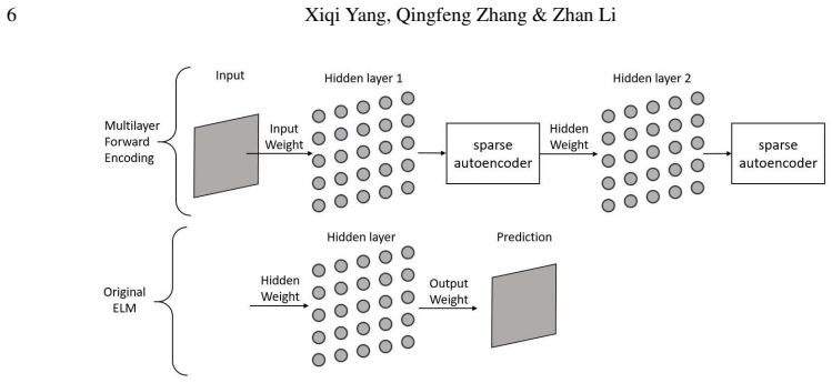
The central object is the hierarchical extreme learning machine (H-ELM): an ELM is a single-hidden-layer network with random input weights whose output weights are solved by least squares, and H-ELM adds sparse-autoencoder layers in front of it to learn compact features without backpropagation. The paper pairs it with a dense conditional random field (DenseCRF), which models all pairs of pixels and is used as a back-end optimizer to smooth the H-ELM's pixel probabilities using image grayscale and spatial proximity. Each pixel is first encoded as a 28-dimensional vector made of nine first-order gradients, nine second-order gradients, and ten Haar-like features, so the learning task is a binary classification of pixels into contour (1) and non-contour (0). The machinery's role is to make training fast (closed-form least squares for the output weights) while the DenseCRF supplies the global consistency that removes spurious interior edges.

What would settle it

Regenerate ground truth by independent manual contour annotation on the same 200 images, then retrain the same H-ELM+DenseCRF pipeline and a stronger deep edge-detection network (for instance a deeper CNN or HED) on the same 130 training images and compare F1 on the 70 test images; if the deep network matches or exceeds 0.58 F1, or if the H-ELM advantage disappears under the new labels, the paper's central claim is unsupported.

Watch

Extended reading notes

Core claim

On its own terms, the paper's discovery is that a deliberately shallow learning pipeline can beat both classical edge detectors and a convolutional network at the specific task of extracting the outer contour of a disk-resolved body in Cassini ISS images. The authors label 200 ISS images semi-automatically by running Canny and manually correcting the result, then train a two-layer sparse-autoencoder feature extractor followed by an ELM classifier on 28 handcrafted features per pixel. After classification, DenseCRF enforces spatial consistency and removes interior contours. The reported numbers are a 0.58 average F1-measure on 70 test images, 0.66 precision, 0.54 recall, and a training time of about 9.004 seconds, against an SVM at 112.270 s, a plain ELM at 7.573 s, and a four-layer CNN at 6138.948 s. The paper concludes that the method is suitable for routine contour detection in Cassini ISS astrometry.

Load-bearing premise

The claim rests on the assumption that the semi-automatic Canny-based labels are a fair ground truth, that the 70 test images represent typical Cassini ISS conditions, and that the shallow CNN used for comparison is a fair representative of deep networks.

Editorial extensions

If this is right

Cassini's archive of more than 400,000 images becomes practical to process for disk-resolved astrometry, since each image takes roughly 7.8 seconds on a commodity CPU after a 9-second training run.
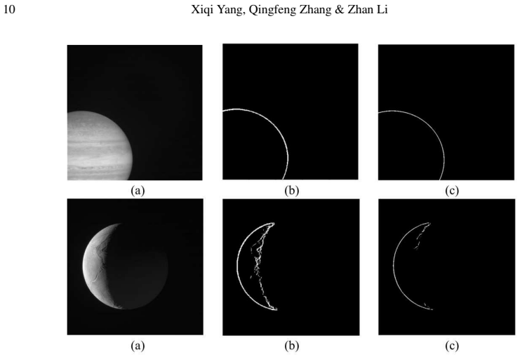
The DenseCRF stage cleanly removes the terminator and other interior boundaries, so the output is a single outer limb suitable for center-of-figure estimates.
The method does not require a GPU or a large labeled corpus, which lowers the barrier for processing future planetary imaging datasets.
The reported precision (0.66) and recall (0.54) show the detector errs toward not marking uncertain pixels, which is the favorable direction when false contour pixels would corrupt center fitting.

Reading between the lines

Editorial extensions of the paper, not claims the author makes directly.

If the labels are unbiased, the same 28-feature H-ELM+DenseCRF recipe should transfer to other disk-resolved solar-system bodies (e.g., Jupiter and its moons) with no architectural change, although the paper does not test this.
The 'beats deep CNN' claim is only as strong as the comparison network: the paper's CNN uses four 3x3 convolution layers, two max-pooling layers, and 28x28 inputs, so a modern edge-detection network trained on the same data might close the gap.
Because the training-time comparison mixes different algorithms on a single laptop CPU, the practical speed advantage could shift when implementations are optimized or run on GPUs; the paper does not report such runs.
A direct test of astrometric value would be to measure how much the detected contours change derived satellite centers compared with manual limb fits; the paper stops at pixel-level F1.

Share X Bluesky LinkedIn Reddit HN

Signed reviews

No signed human review yet.

Editorial analysis

A structured set of objections, weighed in public.

Desk editor's note, referee report, and a circularity audit.

Desk Editor's Note

read the letter

This is a real applied-ML paper, not a methodological breakthrough. The combination of H-ELM with DenseCRF post-processing for contour detection in Cassini ISS images is new in this domain, and the application is well motivated: Cassini returned hundreds of thousands of images, disk-resolved objects produce false star detections in astrometry, and training speed matters. The 9-second training time on a laptop CPU is genuinely attractive, and the DenseCRF step sensibly removes the terminator while keeping the outer contour, which is exactly what center-finding needs. Earlier comparisons against Canny, Sobel, Roberts, Prewitt, SVM, and plain ELM all show reasonable behavior on the example images. Credit where due: the authors know their problem and put together a sensible pipeline.

The soft spots are significant. The headline claim, repeated in the abstract and introduction, is that this method beats 'even deep convolutional neural networks.' But the CNN used for comparison is a 28x28 patch classifier with four 3x3 convolutional layers, two max-pooling layers, and one fully connected layer. That is not a representative modern deep edge detector, not even close to the HED and U-Net architectures the paper itself cites. The comparison conflates model family, input size, and post-processing, so the claim of superiority over deep networks is simply untested. The inconsistency in Table 2 is concrete: the listed F1 values for nine images average to about 0.63, yet the table reports an average of 0.580; precision and recall averages are similarly far off the listed values. That looks like a copy-paste or calculation error, but it undermines confidence in the numbers. There are no error bars, the test set is only 70 images, and no dataset or code is released. The ground truth is semi-automatic Canny with manual correction, which could bias the evaluation, though the authors do acknowledge the terminator-labeling choice.

If taken as a modest engineering contribution, the paper is fine. The central claim needs to be scaled back to 'competitive with a small CNN baseline' or the baselines need to be upgraded to real deep edge detectors. A careful reviewer could fix this, and the corrected tables and error bars are well within reach. I would send this to peer review rather than desk reject, because the problem is real and the method is plausible, but I would expect major revisions. If the authors cannot strengthen the comparison or fix the table, the paper should be published with a much more modest claim or as a short application note.

Referee Report

3 major / 5 minor

Summary. The paper proposes a contour detection method for Cassini ISS images that combines a Hierarchical Extreme Learning Machine (H-ELM) with a Dense Conditional Random Field (DenseCRF) post-processing step. Each pixel is described by 28 hand-crafted features (first-order gradients, second-order gradients, and Haar-like features), classified by an H-ELM whose unsupervised layers are trained with sparse autoencoders, and the resulting probability map is refined by DenseCRF. Experiments on 130 training and 70 test ISS images (512×512, each containing one disk-resolved object) report an average F1-measure of 0.58, a training time of about 9 seconds, and a per-image testing time of about 7.8 seconds. Comparisons are made against Canny/Sobel/Roberts/Prewitt edge operators, SVM, ELM, and a CNN baseline, and the authors claim the method outperforms all of these, including 'even deep convolutional neural network'.

Significance. If the reported results are reliable, the method offers a fast and reasonably accurate contour detector for Cassini ISS images, which is relevant for astrometry and for removing false star detections inside planetary disks. The paper is transparent about the preprocessing, feature set, network structure, and hyperparameter choices, and it reports quantitative comparisons against several baselines. However, the central claim of superiority over deep convolutional neural networks is not supported by the experiments as presented: the CNN baseline is a small patch-based classifier, no error bars or statistical tests are given, and the contribution of DenseCRF is only shown qualitatively. The core H-ELM pipeline is plausible and may be useful for the intended application, but the evidence as it stands does not justify the headline claim about deep networks.

major comments (3)

[§5.3.4, Table 3] The claim in the abstract and Section 1 that the proposed method outperforms 'even deep convolutional neural network' is not supported by the comparison reported in Table 3. The CNN baseline is a patch-based classifier that takes 28×28 image blocks as input and output, with only four 3×3 convolutional layers, two 2×2 max-pooling layers, and one fully connected layer. This is not representative of modern deep convolutional contour detectors such as HED (Xie & Tu 2017) or U-Net, which the introduction itself cites, and it also uses a different input representation (raw patches vs. 28 handcrafted features) and no post-processing. To support the claimed superiority, the authors should provide a comparison with a competitive full-image deep edge detector (or at least a properly tuned CNN on the same input representation), and report error bars so the reader can assess the significance of the difference.
[§5.3.5 and §3] The benefit of DenseCRF post-processing is only demonstrated qualitatively in Figure 10, but it is listed as one of the method's advantages in the conclusion. Since the contribution of the CRF is a load-bearing part of the proposed pipeline, the paper should provide quantitative F1-measure, precision, and recall for H-ELM without DenseCRF on the same test set. Without this ablation, the reader cannot determine how much of the reported improvement over ELM and SVM is due to the CRF rather than to the hierarchical feature learning in H-ELM.
[§5.2, Table 2] No error bars, standard deviations, or confidence intervals are reported for any of the performance metrics. The test set consists of only 70 images, and per-image F1 values among the nine listed examples range from 0.588 to 0.697, indicating substantial variance. Point estimates alone are insufficient to establish that the observed differences between methods are statistically meaningful, especially given the small sample and the large reported gap between the proposed method and the CNN baseline. The authors should report variance or per-image distributions for all methods.

minor comments (5)

[Table 2] The row labeled 'Average' appears to be the mean over the full 70-image test set, but the caption says the table shows results 'in some ISS images' without specifying that the average is over all test images. The mean of the nine listed F1 values is approximately 0.626, not 0.580, which is confusing. Please clarify in the caption that the Average row covers the complete test set.
[§2.2] The paper states that 34 candidate features were designed and 28 were selected based on 'some common senses and some experiments,' but the six omitted features are never described. Please provide the full candidate list and a more explicit feature-selection rationale so the reader can judge whether the chosen set is justified.
[§5.1] The choice of the H-ELM architecture (three hidden layers with 200, 200, and 1000 nodes) is justified only by 'our experiments and comparative analysis' without reporting the results of that analysis. A brief parametric study or a reference to a prior evaluation would make this key design decision more reproducible.
[Throughout] There are multiple typographical and grammatical errors that should be corrected, including 'dont' in §5.3.2, inconsistent 'Harr-like'/'Haar-like' in §2.2.3, and the reference 'Krhenbhl & Koltun' which should read 'Krähenbühl & Koltun'. A careful editing pass is needed.
[Abstract and Conclusions] The phrase 'deep convolutional neural network' is used loosely. The CNN evaluated in §5.3.4 is a shallow patch-based classifier, not a deep full-image network. Please use precise terminology so that the claims match the actual experiments.

Circularity Check

0 steps flagged · score 0.0 of 10

No significant circularity; the H-ELM+DenseCRF contour detector is an empirical construction evaluated on an independent test set.

full rationale

The paper contains no derivation that reduces to its inputs. The method is a supervised pixel classifier: 28 handcrafted features (Sec. 2.2) are fed to H-ELM (Sec. 2.3), whose sparse-autoencoder layers and ELM classifier are standard constructions cited to Tang et al. (2016) and Huang et al. (2006), and DenseCRF post-processing is taken from Krähenbühl and Koltun (2012). Hyperparameters are selected by grid search on the training set (Sec. 5.1), which is ordinary model selection rather than fitting the test result. Labels are semi-automatic Canny plus manual correction (Sec. 4.1); although Canny-derived labels could bias the comparison with Canny, the manual correction and the evaluation on held-out images make this an evaluation-design concern, not circularity. The citation of Yang et al. 2018 as "our previous research" is a self-citation, but it is used only as motivation for the method family, and no load-bearing claim depends on it; H-ELM and DenseCRF are introduced and cited to their original external sources. The concern that the CNN baseline is unrepresentative (four 3x3 convolution layers, 28x28 patches, no CRF, Table 3) is a correctness and fairness critique of the empirical comparison, not circularity under the definition used here. Accordingly, no circular step is identified.

Assumptions & free parameters 4 free parameters · 5 assumptions · 0 invented entities

The paper contributes no new mathematical or physical entities. It relies on existing ML models and a hand-crafted feature set. The main free parameters are hyperparameters and the feature subset, all chosen empirically on the training data.

free parameters (4)

Regularization factor C = 2^18
Chosen by grid search on the training set (Section 5.1); controls the ELM output weight regularization.
Number of hidden layers and nodes = 3 layers: 200, 200, 1000 nodes
Chosen by experiments and comparative analysis (Section 5.1); no theoretical basis.
Under-sampling ratio = 1:4 positive to negative
Chosen after experiments (Section 4.2) to address class imbalance.
Feature set size = 28 of 34 candidate features
Selected based on average accuracy from experiments (Section 2.2); the discarded 6 features are not specified.

assumptions (5)

domain assumption ELM with random input weights and least-squares output weights is a valid classifier
Adopted from Huang et al. 2006, used throughout Section 2.3.1.
domain assumption H-ELM with sparse autoencoders improves feature learning
Adopted from Tang et al. 2016, used in Section 2.3.2.
domain assumption DenseCRF can optimize pixel labels using image gray-level information
Adopted from Krähenbühl and Koltun 2012, used in Section 3.
ad hoc to paper The 28 hand-crafted features are sufficient for contour classification
No theoretical justification; chosen empirically in Section 2.2.
domain assumption The training labels (Canny plus manual correction) are accurate ground truth
Assumed in Section 4.1; all metrics depend on this.

how reviews work

0 comments

Cite this review

Pith. "Pith review of Contour Detection in Cassini ISS images based on Hierarchical Extreme Learning Machine and Dense Conditional Random Field." pith.science (2026). https://pith.science/paper/VPUWDR6P

@misc{pith2026190808279,
  author       = {Pith},
  title        = {Pith review of: Contour Detection in Cassini ISS images based on Hierarchical Extreme Learning Machine and Dense Conditional Random Field},
  year         = {2026},
  howpublished = {\url{https://pith.science/paper/VPUWDR6P}},
  note         = {Machine review of arXiv:1908.08279}
}

read the original abstract

In Cassini ISS (Imaging Science Subsystem) images, contour detection is often performed on disk-resolved object to accurately locate their center. Thus, the contour detection is a key problem. Traditional edge detection methods, such as Canny and Roberts, often extract the contour with too much interior details and noise. Although the deep convolutional neural network has been applied successfully in many image tasks, such as classification and object detection, it needs more time and computer resources. In the paper, a contour detection algorithm based on H-ELM (Hierarchical Extreme Learning Machine) and DenseCRF (Dense Conditional Random Field) is proposed for Cassini ISS images. The experimental results show that this algorithm's performance is better than both traditional machine learning methods such as SVM, ELM and even deep convolutional neural network. And the extracted contour is closer to the actual contour. Moreover, it can be trained and tested quickly on the general configuration of PC, so can be applied to contour detection for Cassini ISS images.

Figures

Figures reproduced from arXiv: 1908.08279 by the authors.

**Figure 1.** A pixels 5×5 neighborhood and its eight directions used in the calculation of first-order and second-order gradient. 2.2 Feature selection Feature selection is an important step before the model training. Appropriate feature selection can make the classifier more robust. In our experiments, 34 candidate features are designed, including image gray level, Hessian feature, Kirsch operator, Robinson operator, Sobel oper… view at source ↗

**Figure 2.** Haar-like features. (1) edge features. (2) line feat [PITH_FULL_IMAGE:figures/full_fig_p004_2.png] view at source ↗

**Figure 3.** The structure of single-hidden-layer ELM. From top t [PITH_FULL_IMAGE:figures/full_fig_p005_3.png] view at source ↗

Figures from the paper (7 more)

**Figure 4.** Figure 4: The network structure of H-ELM. The network includes [PITH_FULL_IMAGE:figures/full_fig_p006_4.png]

**Figure 5.** Figure 5: Contour detection results comparison in Cassini ISS [PITH_FULL_IMAGE:figures/full_fig_p009_5.png]

**Figure 6.** Figure 6: Contour detection results comparison in Cassini ISS [PITH_FULL_IMAGE:figures/full_fig_p009_6.png]

**Figure 7.** Figure 7: Contour detection results comparison in Cassini ISS [PITH_FULL_IMAGE:figures/full_fig_p010_7.png]

**Figure 8.** Figure 8: The CNN architecture in the comparison experiment. [PITH_FULL_IMAGE:figures/full_fig_p011_8.png]

**Figure 9.** Figure 9: Contour detection results comparison in Cassini ISS [PITH_FULL_IMAGE:figures/full_fig_p011_9.png]

**Figure 10.** Figure 10: Contour detection results comparison in Cassini IS [PITH_FULL_IMAGE:figures/full_fig_p012_10.png]

Discussion (0). Continue with ORCID to comment.

Reference graph

Works this paper leans on

27 extracted references · 27 canonical work pages

[1]

2011, IEEE t ransactions on pattern analysis and machine intelligence, 33, 898 2, 8

Arbelaez, P ., Maire, M., Fowlkes, C., & Malik, J. 2011, IEEE t ransactions on pattern analysis and machine intelligence, 33, 898 2, 8

work page 2011
[2]

M., Snchez, J

Barandela, R., V aldovinos, R. M., Snchez, J. S., & Ferri, F. J. 2004, Lecture Notes in Computer Science, 3138, 806 7

work page 2004
[3]

V ., Bowyer, K

Chawla, N. V ., Bowyer, K. W ., Hall, L. O., & Kegelmeyer, W . P . 2002, Journal of Artiﬁcial Intelligence Research, 16, 321 7

work page 2002
[4]

J., Murray, C

Cooper, N. J., Murray, C. D., Lainey, V ., et al. 2014, A&A, 572, A43 1

work page 2014
[5]

2012, Journal o f Geophysical Research, 117, E07005 2

Cornet, T., Bourgeois, O., Moulic, S., et al. 2012, Journal o f Geophysical Research, 117, E07005 2

work page 2012
[6]

2005, IEEE Conference on Computer Vis ion and Pattern Recognition (CVPR 2005), 1, 886 2

Dalal, N., & Triggs, B. 2005, IEEE Conference on Computer Vis ion and Pattern Recognition (CVPR 2005), 1, 886 2

work page 2005
[7]

2006, in , 1964 2

Dollr, P ., Tu, Z., & Belongie, S. 2006, in , 1964 2

work page 2006
[8]

2013, IEEE t ransactions on pattern analysis and machine intelligence, 35, 1915 2

Farabet, C., Couprie, C., Najman, L., & Lecun, Y . 2013, IEEE t ransactions on pattern analysis and machine intelligence, 35, 1915 2

work page 2013

Show all 27 references

[9]

2006, Neurocomputing, 70, 489 4

Huang, G., Zhu, Q., & Siew, C. 2006, Neurocomputing, 70, 489 4

2006
[10]

Y uille, A., Coughlan, J., & Zhu, S

Konishi, S., L. Y uille, A., Coughlan, J., & Zhu, S. 2003, Patt ern Analysis and Machine Intelligence, IEEE Transactions on, 25, 57 2

2003
[11]

2012, Adv

Krhenbhl, P ., & Koltun, V . 2012, Adv. Neural Inf. Process. Syst., 24, 109 6

2012
[12]

2002, Proc ICML, 28 2 6

Lafferty, J., Mccallum, A., & Pereira, F. 2002, Proc ICML, 28 2 6

2002
[13]

2002, in , 900 4

Lienhart, R., & Maydt, J. 2002, in , 900 4

2002
[14]

2018, Research in Astronomy and Astrophysics, 18, 022 1

Liu, B., Y u, J.-Z., & Peng, Q.-Y . 2018, Research in Astronomy and Astrophysics, 18, 022 1

2018
[15]

2015, PloS one, 10, e0134254 4

Mcdonnell, M., Tissera, M., Vladusich, T., van Schaik, A., & Tapson, J. 2015, PloS one, 10, e0134254 4

2015
[16]

Minhas, R., Baradarani, A., Seifzadeh, S., & Wu, Q. M. J. 2010 , Neurocomputing, 73, 1906 4

2010
[17]

2017, Research in Astronomy and Astrophysics, 17, 21 1 R Martin, D., C Fowlkes, C., & Malik, J

Peng, H.-W ., Peng, Q.-Y ., & Wang, N. 2017, Research in Astronomy and Astrophysics, 17, 21 1 R Martin, D., C Fowlkes, C., & Malik, J. 2004, IEEE transactio ns on pattern analysis and machine intelligence, 26, 530 2, 8

2017
[18]

M., Upadhyaya, T

Saheba, S. M., Upadhyaya, T. K., & Sharma, R. K. 2016, IET Imag e Processing, 10, 657 2

2016
[19]

Cooper, N., Lainey, V ., Charnoz, S., & D

Tajeddine, R., J. Cooper, N., Lainey, V ., Charnoz, S., & D. Mu rray, C. 2013, Astronomy and Astrophysics, 551, 129 1

2013
[20]

2015, Astronomy and Astrophysics, 575 1

Tajeddine, R., Lainey, V ., Cooper, N., & Murray, C. 2015, Astronomy and Astrophysics, 575 1

2015
[21]

2016, IEEE Transactions on Neu ral Networks and Learning Systems, 27, 809 6

Tang, J., Deng, C., & Huang, G. 2016, IEEE Transactions on Neu ral Networks and Learning Systems, 27, 809 6

2016
[22]

2015, Geoscience and Remote Sensing, IEEE Transactions on, 53, 1174 4 V apnik, V

Tang, J., Deng, C., Huang, G., & Zhao, B. 2015, Geoscience and Remote Sensing, IEEE Transactions on, 53, 1174 4 V apnik, V . 1998, Statistical Learning Theory, V ol. 108

2015
[23]

2001, in , I 4

Viola, P ., & Jones, M. 2001, in , I 4

2001
[24]

2004, International Journal of Computer Vision, 57, 137 4

Viola, P ., & Jones, M. 2004, International Journal of Computer Vision, 57, 137 4

2004
[25]

2017, International Journal of Computer Vis ion, 125, 1 2 Y ang, X., Zhang, Q., Y ang, X., et al

Xie, S., & Tu, Z. 2017, International Journal of Computer Vis ion, 125, 1 2 Y ang, X., Zhang, Q., Y ang, X., et al. 2018, MA TEC Web of Conferences, 189, 06007 2

2017
[26]

2018, Monthly Notices of the Royal Astronomical Society, 481, 98 1

Zhang, Q., Lainey, V ., Cooper, N., et al. 2018, Monthly Notices of the Royal Astronomical Society, 481, 98 1

2018
[27]

2019, Sci Sin-Phys Mech Astron, 49, 019502 1

Zhang, Q., Xiong, Y ., Peng, Q., et al. 2019, Sci Sin-Phys Mech Astron, 49, 019502 1

2019

Pith tools

Reviewed August 14, 2026 · model on record in the stance chip above.

[1] [1]

2011, IEEE t ransactions on pattern analysis and machine intelligence, 33, 898 2, 8

Arbelaez, P ., Maire, M., Fowlkes, C., & Malik, J. 2011, IEEE t ransactions on pattern analysis and machine intelligence, 33, 898 2, 8

work page 2011

[2] [2]

M., Snchez, J

Barandela, R., V aldovinos, R. M., Snchez, J. S., & Ferri, F. J. 2004, Lecture Notes in Computer Science, 3138, 806 7

work page 2004

[3] [3]

V ., Bowyer, K

Chawla, N. V ., Bowyer, K. W ., Hall, L. O., & Kegelmeyer, W . P . 2002, Journal of Artiﬁcial Intelligence Research, 16, 321 7

work page 2002

[4] [4]

J., Murray, C

Cooper, N. J., Murray, C. D., Lainey, V ., et al. 2014, A&A, 572, A43 1

work page 2014

[5] [5]

2012, Journal o f Geophysical Research, 117, E07005 2

Cornet, T., Bourgeois, O., Moulic, S., et al. 2012, Journal o f Geophysical Research, 117, E07005 2

work page 2012

[6] [6]

2005, IEEE Conference on Computer Vis ion and Pattern Recognition (CVPR 2005), 1, 886 2

Dalal, N., & Triggs, B. 2005, IEEE Conference on Computer Vis ion and Pattern Recognition (CVPR 2005), 1, 886 2

work page 2005

[7] [7]

2006, in , 1964 2

Dollr, P ., Tu, Z., & Belongie, S. 2006, in , 1964 2

work page 2006

[8] [8]

2013, IEEE t ransactions on pattern analysis and machine intelligence, 35, 1915 2

Farabet, C., Couprie, C., Najman, L., & Lecun, Y . 2013, IEEE t ransactions on pattern analysis and machine intelligence, 35, 1915 2

work page 2013