Accelerating small-angle scattering experiments with simulation-based machine learning

Akinori Asahara; Hidekazu Morita; Takuya Kanazawa

REVIEW 3 major objections 5 minor 22 references

Accelerating small-angle scattering experiments with simulation-based machine learning

T0 review · 3 major / 5 minor · reviewed 2026-08-14 · deepseek-v4-flash

Challenge this review Re-run · record.json Download PDF Read on arXiv ↗ Review JSON

Pith's one-line read Adaptive simulation-based sampling cuts SANS measurements by half or more.

desk verdict A clean simulation study of adaptive SANS sampling whose 50–65% savings claim outruns the evidence, because the benchmark is noiseless and the hyperparameters are tuned on the same test set. read the letter →

arxiv 1908.09102 v1 pith:2EQDBL7L submitted 2019-08-24 cond-mat.mtrl-sci cs.LG

Takuya Kanazawa , Akinori Asahara , Hidekazu Morita This is my paper · ORCID

classification cond-mat.mtrl-scics.LG

keywords small-angleneutronscatteringSANSadaptivesamplingsequentialexperimentdesignindirectFouriertransformsimulation-basedmachinelearningmaterialsinformaticsintensitydatabase

topics The Measurement Problem

open problems The Measurement Problem

verification ladder T0 review T1 audit T2 compute T3 formal

The pith

A machine-rendered reading of the paper's core claim, the machinery that carries it, and where it could break.

The reading

This paper proposes that small-angle neutron scattering (SANS) experiments can be accelerated by using a precomputed database of simulated scattering intensities to decide adaptively where to measure next. The authors claim that, in numerical simulations of 100 virtual materials, their two methods reduce the experimental duration needed to reach a given accuracy by 50-65% compared with random sampling, amounting to a factor of 2-3 speedup. The best method, which combines an indirect Fourier transform estimate with a database of similar intensities, reached the accuracy of 40 random measurements in about 13-15 measurements. If this holds in real experiments, it would make sequential SANS measurements substantially cheaper and could extend to small-angle X-ray scattering and other sequential inverse problems.

What carries the argument

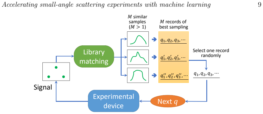
The central machinery is a database of simulated scattering intensities, computed from the forward model I(q) = integral of p(r) F(q,r)^2 dr for a large set of virtual size distributions, together with a normalized similarity measure and the indirect Fourier transform (IFT) that reconstructs p(r) from measured intensities. Method 2's decision rule, q_{n+1} = argmax |I^(1)(q)-I^(2)(q)|/I_0(q), selects the next measurement as the point of maximal disagreement between a database-based intensity guess and an IFT-based intensity guess, thereby targeting the region where the current model is most uncertain. Method 1 instead stores an entire optimized measurement plan per virtual sample and reuses plans from the most similar database entries.

What would settle it

Run the same adaptive-sampling benchmark with Poisson counting noise added to the simulated intensities - for example, setting the detector counts so that the relative error at each q matches typical SANS statistics - and measure the number of measurements needed to reach a fixed L1 distance from the true size distribution; if the reduction versus random sampling drops markedly or disappears, the noiseless result is an artifact of the idealization.

Watch

Extended reading notes

Core claim

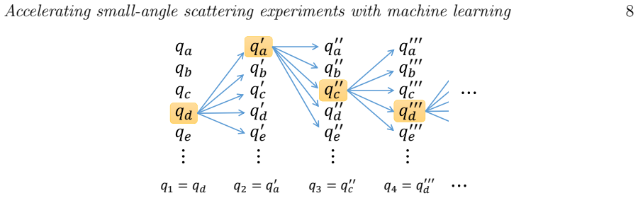
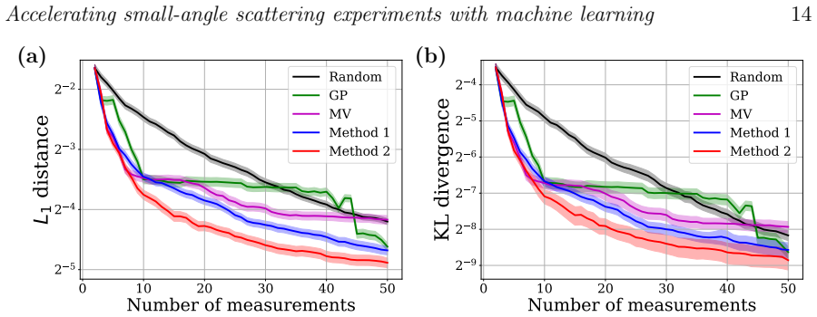
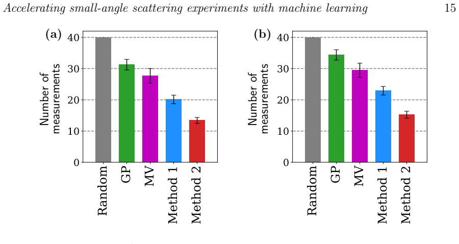
The paper's central claim is that the sequential measurement problem for SANS, where the goal is to reconstruct a size distribution p(r) from scattering intensities I(q) measured at a sparse set of q values, can be solved far more efficiently by adaptive, simulation-based sampling than by non-adaptive random or Gaussian-process baselines. The authors propose two adaptive methods: Method 1 retrieves a precomputed measurement plan for the most similar virtual samples and follows it, while Method 2 predicts future intensities in two independent ways - one from a database of simulated intensities and one from an indirect Fourier transform of the current data - and measures next at the q where the two predictions most strongly disagree. In their noiseless simulations, Method 2 achieved around a 60-65% reduction in the number of measurements required to match random sampling at 40 measurements, and Method 1 achieved roughly a 50% reduction, as measured by both L1 distance and Kullback-Leibler divergence of the reconstructed size distribution.

Load-bearing premise

The benchmark assumes that measurements are noiseless and that the real sample's size distribution comes from the same generative family as the simulated virtual samples, so the measured savings of 50-65% may not transfer to noisy, out-of-distribution experimental conditions.

Editorial extensions

If this is right

SANS experiments could be completed in roughly one-third to one-half the time for the same accuracy, since the tested methods reduce the number of measurements needed by 50-65% relative to random sampling.
Method 2 reached the accuracy of 40 random measurements with about 13.4 measurements by L1 distance and 15.2 by KL divergence, suggesting substantial savings accumulate already in early measurements.
Because small-angle X-ray scattering obeys the same forward relation between size distribution and intensity, the same adaptive planning procedure is expected to accelerate SAXS as well.
The two non-adaptive baselines, Gaussian-process-prioritized sampling and maximal-variance sampling, plateau at low accuracy after an initial fast drop, indicating that fixed or variance-based orderings cannot match the information gain of a forward-model-informed adaptive choice.
Once a database is built, it can be reused across many experiments; the authors note the database for Method 1 costs tens of hours to prepare while Method 2's database takes under an hour.

Reading between the lines

Editorial extensions of the paper, not claims the author makes directly.

In real SANS experiments, Poisson counting noise will likely erode the reported savings: the entire benchmark neglects measurement noise, and both the IFT reconstruction and the pointwise intensity comparison are sensitive to noisy intensities, so the 50-65% reduction is an upper bound for practical settings.
The database approach assumes that the new sample is drawn from the same family of size distributions used to generate virtual samples; out-of-distribution samples such as anisotropic or interacting scatterers would probably degrade both methods, and the paper itself leaves non-spherical scatterers to future work.
The generic principle - measure where two independent forward-model-based predictions diverge most - applies to any inverse problem y = F(x) + n with a known forward model, so the method could be ported to other sequential characterization techniques beyond scattering.
Method 1's dependence on a large precomputed database means its net benefit is only realized after many experiments amortize the database construction cost; Method 2's cheaper database makes it the more practical first choice.

Share X Bluesky LinkedIn Reddit HN

Signed reviews

No signed human review yet.

Editorial analysis

A structured set of objections, weighed in public.

Desk editor's note, referee report, and a circularity audit.

Desk Editor's Note

read the letter

The thing to know: this is a careful numerical demonstration, not a proven experimental speedup. The simulation work is internally consistent and the methods are described well enough to reproduce the ideas, but the abstract's "experimental duration reduced by 50–65%" framing invites a stronger reading than the evidence supports.

What is genuinely new: applying adaptive, database-driven measurement planning to SANS appears to be a new application, and the problem formulation is clear. Method 2 — comparing an IFT-based prediction against a nearest-neighbor database average and measuring the next q at their maximal normalized disagreement — is simple but sensible. The benchmark is also fairly constructed: the IFT setup is common to all methods, 100 virtual samples are averaged, standard deviations are reported, and the GP and MV baselines give the proposed methods a real run for their money. The authors also deserve credit for being explicit about the noiseless assumption and about the computational cost of building the Method 1 database.

The soft spots are the usual ones, but they are not minor. First, Section 3 states that noise is neglected "for simplicity," and the whole benchmark inherits that. Real SANS is dominated by counting statistics, and both the similarity score (20) and the acquisition rule (24) compare pointwise intensities, dividing by a reference intensity. In the presence of Poisson noise, these quantities develop a statistical component that can dominate the disagreement signal, especially where the intensity is small. So the 2–3× savings are a property of the noiseless, same-generator synthetic benchmark, not a demonstrated property of SANS experiments. The authors note that real tests are future work, but the conclusion leans on the stronger claim.

Second, the hyperparameters M = 3 for Method 1 and K'' = 12 for the MV baseline were selected by peeking at the same 100 virtual samples used for the headline comparison, with no independent validation split. That inflates the reported gains relative to what one should expect on a genuinely new sample. This is fixable.

Third, no code or data were released, so the simulation itself cannot be independently checked. That matters less than the noise issue, but it is a real obstacle.

Bottom line: the central simulation claim — that these adaptive methods outperform the stated baselines in the described setting — holds up. The extension to real experiments does not yet. This paper is for people working on SANS/SAXS measurement planning or on active learning for physical measurements generally. It deserves serious refereeing, but a referee should send it back for either a noise-robust simulation or a real experiment, plus a proper validation split. I would not cite it as evidence for experimental speedups yet.

Referee Report

3 major / 5 minor

Summary. The manuscript addresses adaptive measurement planning for small-angle neutron scattering (SANS). The authors assume the scattered intensity is given by I(q) = ∫ p(r) F(q,r)^2 dr with a spherical form factor, and they propose two simulation-based strategies. Method 1 precomputes a greedy optimal measurement plan for each virtual sample, stores the plans in a database, and during an experiment retrieves the plan of the M most similar database samples. Method 2 stores only simulated intensities, forms two independent predictions of unmeasured intensities—one from a database nearest-neighbor average and one from an indirect Fourier transform (IFT) of the measured data—and measures next at the q of maximum normalized disagreement. The methods are benchmarked on 100 virtual samples drawn from the same generator as the database, against random sampling, a Gaussian-process-based fixed ordering, and a maximal-variance baseline. The authors report that Method 1 and Method 2 reach the discrepancy of 40 random measurements in about 20 and 13–15 measurements, respectively, which they translate into a 50–65% reduction in experimental duration.

Significance. If the results survive more realistic noise and distribution-shift tests, this is a useful contribution to adaptive experimental design in scattering science. The numerical comparison is careful in several respects: all methods share the same IFT evaluation pipeline, the database and test samples are drawn from a common generative model, 100 virtual samples are averaged, and standard deviations are reported for the main metric. The paper is also honest that this is a numerical study and that real SANS/SAXS tests are future work. The central limitation is that the benchmark is noiseless and in-distribution; because the abstract and conclusions state the outcome in terms of 'experimental duration,' the practical significance as written exceeds what the simulations can establish.

major comments (3)

[Section 3; Eq. (20); Eq. (24); Table 1] The paper's headline claim of a 50–65% reduction in 'experimental duration' is not supported by the noiseless benchmark. Section 3 explicitly says noise is neglected and that in practice noise can be suppressed by extending measurement duration, but duration is exactly the resource the abstract claims to save. Table 1 counts noiseless measurements, not time. Under counting statistics, the time needed at each q is set by the required signal-to-noise ratio, and the acquisition rules in Eqs. (20) and (24) divide intensity differences by a reference intensity I0(q); wherever I0(q) is small, generally at high q, the statistical component of these ratios can dominate the model-disagreement signal. The reported factor 2–3 is therefore a property of the noiseless synthetic benchmark, not a demonstrated property of SANS experiment duration. I ask for either a simulation with Poisson noise and an explicit integration-time model, or a revised abstract and conclusions that claim only a reduction in the number of noiseless measurements.
[Section 5.1; Section 5.2] Hyperparameters M=3 for Method 1 and K''=12 for the MV baseline are reported as empirically best, apparently on the same 100 virtual samples used for the benchmark. The text states 'Empirically, we found that M = 3 was most effective' and 'we tested K'' = 3, 6, 12, 24 and found that K'' = 12 performed the best.' If these values were selected on the same test samples, the averaged curves in Figure 6 and the entries in Table 1 are optimistically biased, and the comparison with the MV baseline is not on equal footing. Please clarify whether a separate validation set or a nested evaluation was used, or report the sensitivity of the results to M and K''.
[Section 5.1, Eqs. (25)–(27); Section 6] The database and the 100 test samples are generated from the same distribution family, so the similarity searches in Method 1 and Method 2 are evaluated entirely in distribution. Real SANS samples need not lie in this family, and the performance gain depends on the database containing close neighbors. A robustness experiment in which the database and test distributions differ (for example, log-normal or Schulz size distributions, or a perturbed version of Eq. (25)) would substantially strengthen the claim that the methods accelerate actual SANS experiments. As written, the conclusion that SANS experiments can be 'sped up by a factor of 2–3' should be scoped to same-distribution virtual samples.

minor comments (5)

[Section 5.1] The notation 'K = 102' and 'K > 102' appears to mean 10^2; as printed, K = 102 is a specific integer and the following sentence is confusing. Please typeset the powers of ten correctly.
[Eqs. (20), (24); Figure 5] The reference intensity I0(q) is used in the similarity measure and in the acquisition function but is never specified. Please state how I0(q) is chosen in the numerical experiments, since the behavior of both methods depends on it.
[Reference [19]] The author name 'Spalzzi' in Reference [19] appears misspelled; the usual spelling is 'Spalazzi.' Please check.
[Section 2; Section 4] The toy problem labels the two approaches 'deductive' and 'inductive,' and the text then says that Method 1 for SANS is akin to the toy's inductive method while Method 2 for SANS is hybrid. This reversal is easy to misread; a short mapping table or a change of terminology would improve clarity.
[Figure 6; Table 1] Please state explicitly whether the shaded bands are standard deviations over the 100 virtual samples or standard errors, and describe how the per-sample number of measurements to reach the threshold discrepancy is computed (for example, by interpolation between integer measurement counts).

Circularity Check

0 steps flagged · score 0.0 of 10

No significant circularity: acquisition rules never access the test sample's true size distribution, and no load-bearing self-citation chain is present.

full rationale

The paper's derivation chain is self-contained in the sense relevant to circularity. The forward model (14) and IFT estimator (15)-(16) are standard, independent inputs; the acquisition rules (20) and (24) are computed from measured intensities and database intensities only. In Method 1, the database plans are optimized offline against the true p_k of database samples, but at deployment the next q is selected by intensity similarity, not by the target p. In Method 2, the next q is chosen by maximal disagreement between an IFT-based prediction and a database average; the true p(r) of the test sample is never used to choose q, only to compute the evaluation metrics (17)-(18). The benchmark is in-distribution and noiseless, which limits external validity, but that is a generalization/robustness concern rather than a circular reduction. There are no load-bearing self-citations: references are standard methodological sources (Glatter, Bishop, Rasmussen, etc.). The acknowledged noiseless assumption and the deferral of real experiments to future work weaken the strength of the '50-65% duration reduction' claim, but do not make the numerical comparison true by construction.

Assumptions & free parameters 5 free parameters · 5 assumptions · 0 invented entities

The central claim rests on the forward scattering model, the chosen virtual-material generator, the noiseless approximation, and several algorithm hyperparameters selected on the same benchmark. No new physical entities are postulated. The main tuning burden is the empirical selection of M and K'' on the test samples, plus the unspecified reference intensity I0.

free parameters (5)

IFT regularization coefficient lambda = 1e-3
Chosen by hand in Section 5.1; it controls the smoothness penalty in all IFT reconstructions and therefore shapes the error metric for all five methods.
Number of similar samples M in Method 1 and Method 2 = 3
Section 5.1 reports that M=3 was found most effective; this was selected empirically on the same benchmark samples with no separate validation set.
Number of similar samples K'' in the MV baseline = 12
Section 5.1 states K''=12 performed best among 3, 6, 12, and 24; this tuning uses the same test data and could inflate the baseline's apparent performance.
Reference intensity I0(q) = unspecified
Used to normalize similarity in eq. (20) and selection in eq. (24); it is called arbitrary but never specified, and the results could depend on this choice.
Virtual sample generator parameters = alpha_i uniform in [-1,1], beta_j uniform in [0,2]
These define the family of size distributions in eq. (25); the benchmark only tests this family, so the results are conditional on this generative prior.

assumptions (5)

domain assumption Forward model: I(q) = integral of p(r) F(q,r)^2 dr for polydisperse spheres (eq. 14)
All simulations and IFT inference assume spherical scatterers with no background or instrumental smearing.
domain assumption Virtual materials from eq. (25)-(27) are representative of real SANS samples
Database construction and the 100 test samples both use this generative family; no real experimental data are used.
domain assumption Measurement noise can be neglected
Section 3 explicitly neglects noise and argues that longer counting can suppress it; this is untested in the benchmarks and is a central limitation for real experiments.
domain assumption IFT with 80 basis functions and the chosen regularization yields a reliable estimate of the size distribution
All methods share this reconstruction step; its bias affects both the reported discrepancy and the next-point selection.
domain assumption The database and test samples are generated from the same model
Method 2's success is demonstrated only in-distribution; Section 5.2 attributes success to database size and normalized similarity, not to robustness under distribution shift.

how reviews work

0 comments

Cite this review

Pith. "Pith review of Accelerating small-angle scattering experiments with simulation-based machine learning." pith.science (2026). https://pith.science/paper/2EQDBL7L

@misc{pith2026190809102,
  author       = {Pith},
  title        = {Pith review of: Accelerating small-angle scattering experiments with simulation-based machine learning},
  year         = {2026},
  howpublished = {\url{https://pith.science/paper/2EQDBL7L}},
  note         = {Machine review of arXiv:1908.09102}
}

read the original abstract

Making material experiments more efficient is a high priority for materials scientists who seek to discover new materials with desirable properties. In this paper, we investigate how to optimize the laborious sequential measurements of materials properties with data-driven methods, taking the small-angle neutron scattering (SANS) experiment as a test case. We propose two methods for optimizing sequential data sampling. These methods iteratively suggest the best target for the next measurement by performing a statistical analysis of the already acquired data, so that maximal information is gained at each step of an experiment. We conducted numerical simulations of SANS experiments for virtual materials and confirmed that the proposed methods significantly outperform baselines.

Figures

Figures reproduced from arXiv: 1908.09102 by the authors.

**Figure 1.** Small-angle neutron scattering experiment. scatterers in the sample. If a scatterer is a homogeneous sphere of radius r, the form factor is given by [13] F(q, r) = sin(qr) − qr cos(qr) (qr) 3 . (13) If the ensemble of scatterers consists of spheres of various sizes following a probability distribution p(r), then we have I(q) = Z ∞ 0 dr p(r)F(q, r) 2 (14) where the overall multiplicative factor on the right hand side… view at source ↗

**Figure 2.** Greedy optimization of the measurement plan. where the pair of the scattering intensity and the best plan is stored for every sample. This completes the first step of Method 1. An optimal plan Qk for a sample k can be generated incrementally as depicted in [PITH_FULL_IMAGE:figures/full_fig_p008_2.png] view at source ↗

**Figure 3.** Summary of Method 1. In Method 1 it is essential that the similarity search over D works accurately. This hinges on how the similarity of two scattering data, I1(q) and I2(q), is defined. A naive definition such as P i |I1(qi)−I2(qi)| fails severely, because the scattering intensity grows exponentially toward small q, and thus, contributions from the smallest q easily dominate the above sum. We found it most useful … view at source ↗

Figures from the paper (6 more)

**Figure 4.** Figure 4: Summary of Method 2. the best way to discriminate among pα(r), pβ(r), · · · and p(r)? As the distributions themselves are not observable, we have to compare their scattering intensities. In practice, it is difficult if not impossible to construct pα(r), pβ(r), · · · ou…

**Figure 5.** Figure 5: Ten examples of randomly generated size distributions (left) and their scattering intensities normalized by a reference intensity (right). too expensive for our available resources, k whereas increasing K0 further was feasible but did not bring any performance improvem…

**Figure 6.** Figure 6: Discrepancy as measured by (a) L1 distance and (b) Kullback–Leibler divergence for the five methods, averaged over 100 virtual samples. “GP” and “MV” indicate the methods based on the Gaussian process and maximal variance, respectively. Each color band represents one s…

**Figure 7.** Figure 7: Average number of measurements required for each method to reach the same discrepancy as that of random sampling with 40 measurements. The discrepancy was measured by (a) L1 distance and (b) Kullback–Leibler divergence. Each error bar represents one standard deviation.…

**Figure 8.** Figure 8: Dissection of Method 2. One cycle of the procedure starts from (1) measurement and ends by (6) comparison. See the main text for more details. estimate p?(r), but the discrepancy cannot be calculated without knowing ptrue. So we next turn our focus to comparing scatter…

**Figure 9.** Figure 9: Example of a measurement process with Method 2. The left column is the scattering intensity and the right column is the associated size distribution (both the ground truth and the predicted one). The number of sampled points is 4 (top row), 6 (middle row) and 12 (botto…

Discussion (0). Continue with ORCID to comment.

Reference graph

Works this paper leans on

22 extracted references · 19 canonical work pages

[1]

K. Rajan. Materials informatics. Materials Today, 8:38, 2005

work page 2005
[2]

Lookman, F

T. Lookman, F. J. Alexander, and K. Rajan, editors. Information Science for Materials Discovery and Design, volume 225 of Springer Series in Materials Science . Springer, Switzerland, 2016

work page 2016
[3]

Ramprasad, R

R. Ramprasad, R. Batra, G. Pilania, A. Mannodi-Kanakkithodi, and C. Kim. Machine learning in materials informatics: recent applications and prospects. npj Computational Materials , 3:54, 2017

work page 2017
[4]

Y. Liu, T. Zhao, W. Ju, and S. Shi. Materials discovery and design using machine learning. Journal of Materiomics , 3:159, 2017

work page 2017
[5]

K. T. Butler, D. W. Davies, H. Cartwright, O. Isayev, and A. Walsh. Machine learning for molecular and materials science. Nature, 559:547, 2018

work page 2018
[6]

J. E. Gubernatis and T. Lookman. Machine learning in materials design and discovery: Examples from the present and suggestions for the future. Phys. Rev. Materials , 2:120301, 2018. Accelerating small-angle scattering experiments with machine learning 19

work page 2018
[7]

G. R. Schleder, A. C. M. Padilha, C. M. Acosta, M. Costa, and A. Fazzio. From DFT to machine learning: recent approaches to materials science–a review. J. Phys.: Mater. , 2:032001, 2019

work page 2019
[8]

A. Seko, A. Togo, H. Hayashi, K. Tsuda, L. Chaput, and I. Tanaka. Prediction of Low-Thermal- Conductivity Compounds with First-Principles Anharmonic Lattice-Dynamics Calculations and Bayesian Optimization. Physical Review Letters, 115:205901, 2015

work page 2015

Show all 22 references

[9]

P. I. Frazier and J. Wang. Bayesian Optimization for Materials Design. arXiv:1506.01349, 2015

2015 arXiv
[10]

T. Ueno, T. D. Rhone, Z. Hou, T. Mizoguchi, and K. Tsuda. COMBO: An eﬃcient Bayesian optimization library for materials science. Materials Discovery, 4:18, 2016

2016
[11]

Lookman, P

T. Lookman, P. V. Balachandran, D. Xue, J. Hogden, and J. Theiler. Statistical inference and adaptive design for materials discovery. Current Opinion in Solid State and Materials Science , 21(3):121, 2017

2017
[12]

L. A. Feigin and D. I. Svergun. Structure Analysis by Small-Angle X-Ray and Neutron Scattering . Springer, New York, 1987

1987
[13]

S. Jaksch. Small-Angle Scattering. arXiv:1901.07353, 2019

1901 arXiv
[14]

C. M. Bishop. Pattern Recognition and Machine Learning. Springer, 2006

2006
[15]

O. Glatter. A New Method for the Evaluation of Small-Angle Scattering Data. Journal of Applied Crystallography, 10:415, 1977

1977
[16]

P. B. Moore. Small-angle scattering. Information content and error analysis. Journal of Applied Crystallography, 13:168, 1980

1980
[17]

Hansen and J

S. Hansen and J. S. Pedersen. A Comparison of Three Diﬀerent Methods for Analysing Small- Angle Scattering Data. Journal of Applied Crystallography , 24:541, 1991

1991
[18]

Muthig, S

M. Muthig, S. Prevost, R. Orglmeister, and M. Gradzielski. Indirect Fourier transform in the context of statistical inference. Acta Crystallographica, A72:557, 2016

2016
[19]

L. Spalzzi. A Survey on Case-Based Planning. Artiﬁcial Intelligence Review, 2001

2001
[20]

R. S. Sutton and A. G. Barto. Reinforcement Learning: An Introduction . The MIT Press, Cambridge, Second edition, 2018

2018
[21]

Pedregosa, G

F. Pedregosa, G. Varoquaux, A. Gramfort, V. Michel, B. Thirion, O. Grisel, M. Blondel, P. Prettenhofer, R. Weiss, V. Dubourg, J. Vanderplas, A. Passos, D. Cournapeau, M. Brucher, M. Perrot, and E. Duchesnay. Scikit-learn: Machine learning in Python. Journal of Machine Learning...

2011
[22]

C. E. Rasmussen and C. K. Williams. Gaussian Process for Machine Learning . MIT Press, Cambridge, 2006

2006

Pith tools

Reviewed August 14, 2026 · model on record in the stance chip above.

[1] [1]

K. Rajan. Materials informatics. Materials Today, 8:38, 2005

work page 2005

[2] [2]

Lookman, F

T. Lookman, F. J. Alexander, and K. Rajan, editors. Information Science for Materials Discovery and Design, volume 225 of Springer Series in Materials Science . Springer, Switzerland, 2016

work page 2016

[3] [3]

Ramprasad, R

R. Ramprasad, R. Batra, G. Pilania, A. Mannodi-Kanakkithodi, and C. Kim. Machine learning in materials informatics: recent applications and prospects. npj Computational Materials , 3:54, 2017

work page 2017

[4] [4]

Y. Liu, T. Zhao, W. Ju, and S. Shi. Materials discovery and design using machine learning. Journal of Materiomics , 3:159, 2017

work page 2017

[5] [5]

K. T. Butler, D. W. Davies, H. Cartwright, O. Isayev, and A. Walsh. Machine learning for molecular and materials science. Nature, 559:547, 2018

work page 2018

[6] [6]

J. E. Gubernatis and T. Lookman. Machine learning in materials design and discovery: Examples from the present and suggestions for the future. Phys. Rev. Materials , 2:120301, 2018. Accelerating small-angle scattering experiments with machine learning 19

work page 2018

[7] [7]

G. R. Schleder, A. C. M. Padilha, C. M. Acosta, M. Costa, and A. Fazzio. From DFT to machine learning: recent approaches to materials science–a review. J. Phys.: Mater. , 2:032001, 2019

work page 2019

[8] [8]

A. Seko, A. Togo, H. Hayashi, K. Tsuda, L. Chaput, and I. Tanaka. Prediction of Low-Thermal- Conductivity Compounds with First-Principles Anharmonic Lattice-Dynamics Calculations and Bayesian Optimization. Physical Review Letters, 115:205901, 2015

work page 2015