REVIEW 2 major objections 6 minor 13 references
Almost Tune-Free Variance Reduction
T0 review · 2 major / 6 minor · reviewed 2026-08-14 · deepseek-v4-flash
Pith's one-line read This paper claims that SVRG and SARAH can be made almost tune-free using Barzilai-Borwein step sizes, weighted averaging, and an inner-loop length $m_s = c/(\mu\eta_s)$, with proven linear convergence.
desk verdict Solid theoretical core with a genuinely new averaging scheme, but the 'almost tune-free' claim rests on boundary parameter choices that violate the paper's own theorems and are supported only by three datasets without error bars or code. read the letter →
The pith
A machine-rendered reading of the paper's core claim, the machinery that carries it, and where it could break.
The reading
What carries the argument
The load-bearing object is the estimate sequence, a chain of quadratic surrogate functions $\Phi_k(x)$ built inside each inner loop from the algorithm's gradient estimates. Starting from $\Phi_0(x)=\Phi_0^*+(\mu_0/2)\|x-x_0\|^2$, each step defines $\Phi_k$ recursively from $\Phi_{k-1}$ and the current estimate $v_{k-1}$, with $\delta_k=\mu_k\eta$; this sequence supplies both the weighted-averaging probabilities and the contraction factors $\lambda_{\mathrm{SVRG}}$ and $\lambda_{\mathrm{SARAH}}$. Around it, three components work together: the Barzilai-Borwein step size $\eta_s$ computed from the two previous outer iterates, which removes step-size tuning; the W-Avg rule, which favors early inner-loop iterates whose gradient estimates carry less noise; and the rule $m_s = c/(\mu\eta_s)$, which keeps the product of step size and inner-loop length in the theoretically favorable regime.
What would settle it
Run BB-SARAH with $\theta_\kappa=\kappa$, $c=1$, and W-Avg on a strongly convex smooth finite-sum problem, tracking $\mathbb{E}[\|\nabla f(\tilde{x}_s)\|^2]$ as $\eta_s$ ranges through its allowed interval $[1/(\theta_\kappa L), 1/(\theta_\kappa \mu)]$; any divergence, or measured IFO complexity worse than $O((n+\kappa^2)\ln(1/\epsilon))$, would falsify the almost tune-free claim.
Extended reading notes
Core claim
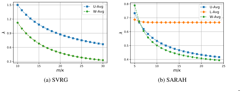
On its own terms, the paper's discovery is that averaging choices inside a double-loop variance-reduction method are performance-critical, and that the right averaging can be read off an estimate-sequence construction. For SVRG, weights $p_s^k = (1-\mu\eta)^{m-k-1}/q$ for $k=1,\dots,m-1$ yield a contraction factor $\lambda_{\mathrm{SVRG}}$ that improves on uniform averaging, giving linear convergence with $O((n+\kappa)\ln(1/\epsilon))$ IFO complexity. For SARAH, whose gradient estimate is biased, weights $p_s^k$ proportional to $1-(1-\mu\eta)^{m-k-1}$ for $k=0,\dots,m-2$ yield linear convergence in $\mathbb{E}[\|\nabla f(\tilde{x}_s)\|^2]$ under Assumptions 1 and 4. The estimate-sequence machinery is then combined with BB step sizes and the adaptive inner-loop length $m_s=c/(\mu\eta_s)$ to produce almost tune-free BB-SVRG and BB-SARAH, with the BB variants proven at $O((n+\kappa^2)\ln(1/\epsilon))$ IFO calls.
Load-bearing premise
The practical claim rests on the empirical premise that the boundary constants $\theta_\kappa=4\kappa$ (SVRG), $\theta_\kappa=\kappa$ (SARAH), and $c=1$ with $m_s=c/(\mu\eta_s)$ keep the algorithm convergent even though these choices fall outside the strict conditions of the theorems (which require $\theta_\kappa>4\kappa$ or $\theta_\kappa>\kappa$ and $m=O(\kappa^2)$); the paper's only support for this premise is that no divergence showed up in its experiments. If that empirical premise fails, the almost tune-free claim collapses.
Editorial extensions
If this is right
- SVRG with W-Avg converges linearly in objective value at $O((n+\kappa)\ln(1/\epsilon))$ IFO complexity, matching the order of tuned SVRG without requiring a searched step size.
- SARAH with W-Avg converges linearly in $\mathbb{E}[\|\nabla f(\tilde{x}_s)\|^2]$ at $O((n+\kappa)\ln(1/\epsilon))$ IFO complexity under smooth strongly convex finite-sum assumptions, extending estimate-sequence analysis to biased gradient estimates.
- BB-SVRG and BB-SARAH with $m=O(\kappa^2)$ and $\theta_\kappa=4\kappa$ or $\kappa$ have $O((n+\kappa^2)\ln(1/\epsilon))$ complexity, so when $\kappa^2$ is no larger than $n$, the automatic step size costs almost nothing in theory.
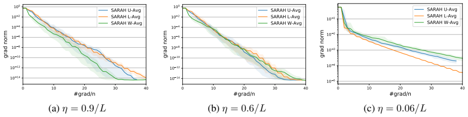
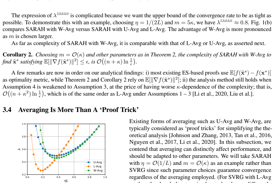
- Averaging matters empirically: W-Avg beats L-Avg and U-Avg when the step size or inner-loop length is large, while small step sizes favor L-Avg, so parameter choice should be coordinated across step size, inner-loop length, and averaging.
- With the fixed boundary constants $\theta_\kappa=4\kappa$ (SVRG), $\theta_\kappa=\kappa$ (SARAH), and $c=1$, the proposed schemes match or outperform tuned SVRG and SARAH on the datasets tested (a9a, rcv1, real-sim).
Reading between the lines
- An implicit consequence of $m_s=c/(\mu\eta_s)$ is that the product $\mu\eta_s m_s$ is constant, so the per-outer-loop contraction factor is kept away from the unstable regime across the whole range of BB step sizes; the paper hints at this but does not state it as a theorem.
- The W-Avg weights have a natural early-ending interpretation: they down-weight late inner iterates whose gradient estimates carry the most variance, which suggests the same adjustment might improve other variance-reduction schemes (e.g., SAGA or loopless SVRG) whenever step sizes are large.
- A direct test of the almost-tune-free claim would be to run BB-SARAH with $\theta_\kappa=\kappa$ and $c=1$ on a strongly convex smooth finite-sum problem and record whether divergence ever occurs when $\eta_s$ is near its smallest value $1/(\theta_\kappa L)$; the paper's experiments report no divergence but do not cover all worst-case regimes.
- The estimate-sequence proof for biased gradient estimators could be reused to produce averaging rules for other recursive estimators, such as SPIDER or SNVRG, whose bias terms have a similar telescoping structure.
Signed reviews
Editorial analysis
A structured set of objections, weighed in public.
Referee Report
Summary. The paper studies SVRG and SARAH for strongly convex finite-sum minimization and proposes weighted averaging (W-Avg) derived from an estimate-sequence analysis. Theorem 1 and Corollary 1 give SVRG with W-Avg linear convergence and O((n+κ)ln(1/ε)) IFO complexity under Assumptions 1-3; Theorem 2 and Corollary 2 give an analogous result for SARAH with W-Avg, measured in E[||∇f(x̃_s)||²], under Assumptions 1 and 4. The paper then analyzes Barzilai-Borwein step sizes for SVRG and SARAH with fixed inner-loop length m=O(κ²) (Propositions 1-2), and proposes an adaptive inner-loop rule m_s=c/(μη_s) with c=1 and θ_κ=4κ (SVRG) or θ_κ=κ (SARAH), marketed as 'almost tune-free.' Numerical experiments on three LIBSVM datasets compare the resulting methods with tuned SVRG and SARAH.
Significance. The estimate-sequence machinery is a real methodological contribution: it extends ES analysis to SARAH's biased gradient estimator and yields provably tighter theoretical rates for W-Avg, and the fixed-m BB variants come with complete proofs. The paper also makes a credible empirical case that averaging is more than a proof trick. However, the headline 'almost tune-free' claim is not established by the theorems: the implemented boundary parameters (θ_κ=4κ or κ, c=1) lie outside the regime covered by Propositions 1-2, and the only support for that regime is three datasets and an anecdotal 'no divergence has been observed' statement. The appendix proofs are organized and appear internally consistent; the central gap is between the proved propositions and the implemented algorithm. If the boundary regime can be proven or convincingly validated across a much broader range of conditioning and random seeds, the contribution would be significant.
major comments (2)
- [4.3, Eq. (9), Propositions 1-2] The implemented 'tune-free' parameters are outside the proven regime. Since η_s ≤ 1/(θ_κ μ) by Eq. (8), the adaptive rule m_s = c/(μη_s) with c=1 gives m_s = θ_κ = O(κ) at the upper end of the step-size range, whereas Propositions 1 and 2 require m=O(κ²) and strict inequalities θ_κ>4κ (SVRG) or θ_κ>κ (SARAH). At the boundary the contraction bounds fail: for BB-SARAH with θ_κ=κ, m_s=κ and η_s=1/(κμ), the U-Avg rate in the proof of Proposition 2 equals 1/(μη_s m_s)+η_s L/(2−η_s L)=1+1=2, so λ_s>1; for BB-SVRG with θ_κ=4κ and m_s=4κ, the W-Avg bound in the proof of Proposition 1 contains the term 2κ/θ_κ/(1−2κ/θ_κ)=1, hence λ_s≥1. The paper's own caveat in Sec. 4.3 ('the selection of these parameters violates slightly the theoretical guarantee... no divergence has been observed') understates this gap: the violation is not a small constant but an order-of-magnitude difference in m. The central practical claim therefore currently rests on an unproven empirical premise. I ask the authors to either extend the analysis to cover θ_κ=κ, 4κ with m_s=θ_κ (e.g., a sharpened W-Avg contraction with m=O(κ)), or restructure the claim and support it with systematic experiments across conditioning regimes.
- [5, Table 1] The empirical validation of the boundary regime is too thin for the generality of the 'almost tune-free' claim. The experiments use three datasets, all with the same regularized logistic loss, no reported values of L or κ, no error bars or repeated-seed statistics, and no released code. Because Sec. 4.3 explicitly replaces a proof with 'no divergence has been observed,' the revision should report κ for each dataset, include a large-κ example (e.g., κ²≫n, a regime where the paper itself predicts BB slowdown in Sec. 4.2), average over multiple random seeds and starting points, and specify the exact BB implementation including any safeguards for the denominator in Eq. (7). Without this, the claim that the parameter choices are robust across problems is not supported.
minor comments (6)
- [Assumption 1 and Introduction] 'L-Lipchitz' should be 'L-Lipschitz'; the same typo appears in the Introduction.
- [Appendix A.1] In the proof of Lemma 2, 'Hession' should be 'Hessian.'
- [Corollary 2 proof] The last sentence of the proof says 'λSVRG≤0.75' but the quantity analyzed is λSARAH.
- [Figure 5] The legend of Figure 5(b) appears to list 'SVRG' twice; it should include 'BB-SVRG.'
- [4.3, Eq. (9)] The paper should clarify what 'almost tune-free' means regarding problem constants: Eq. (9) requires μ, and θ_κ=κ requires L/μ, but no procedure for estimating or obtaining these constants is discussed; Table 1 reports only μ.
- [References] The bibliographic entry for Liu et al. lacks a year; please complete the reference.
Circularity Check
No significant circularity: the W-Avg convergence proofs are self-contained; the admitted boundary-parameter violation is a correctness/robustness caveat, not a circular reduction.
full rationale
The central derivation is self-contained. Theorem 1 and Theorem 2 derive the W-Avg contraction factors λSVRG and λSARAH from the estimate-sequence machinery (Lemma 2), the MSE bounds of Lemma 1, and the SARAH variance bound of Lemma 5; the averaging weights are closed-form functions of μ, η, and m, not quantities fitted to the target convergence. Corollaries 1 and 2 then choose explicit η and m=O(κ) to read off O((n+κ)ln(1/ε)) IFO complexity. The BB analysis (Propositions 1 and 2) plugs the same in-paper rates into the range bound 1/(θκL) ≤ η_s ≤ 1/(θκμ), again without importing the conclusion. The final tune-free recipe (Section 4.3) is an adaptive heuristic: m_s = c/(μη_s) with θκ=κ/4κ and c=1. The paper explicitly concedes a theory-practice gap: 'Although the selection of these parameters violates slightly the theoretical guarantee, its merits lie in the simplicity. And in our experiments, no divergence has been observed by these parameter selections.' That is an empirical robustness claim about a boundary regime (m_s=O(κ) instead of O(κ²), θκ at the strict-inequality boundary), and as such it is a correctness risk, not a circularity. Self-citations to [Li et al., 2020] (L-Avg SARAH) and to the authors' technical note [Li and Giannakis, 2019] (extensions) are not load-bearing for the W-Avg convergence theorems, which are proved in this paper; the L-Avg option in Proposition 2 is not the averaging used in the proposed tune-free algorithms. No prediction is equivalent by construction to a fitted input, and no load-bearing argument reduces to a self-citation chain.
Assumptions & free parameters
free parameters (2)
- θκ =
4κ (BB-SVRG), κ (BB-SARAH)
- c =
1
assumptions (6)
- domain assumption Each f_i has L-Lipschitz gradient (Assumption 1).
- domain assumption Each f_i is convex (Assumption 2).
- domain assumption f is μ-strongly convex (Assumption 3).
- domain assumption Each f_i is μ-strongly convex (Assumption 4).
- domain assumption Cited MSE bounds (Lemma 1 from Johnson & Zhang and Nguyen et al.; Lemma 5 from Nguyen et al.) hold.
- ad hoc to paper Heuristic parameter choices (θκ boundary values and c = 1) make the tune-free algorithm converge in practice.
Cite this review
Pith. "Pith review of Almost Tune-Free Variance Reduction." pith.science (2026). https://pith.science/paper/HMIRZ6BR
@misc{pith2026190809345,
  author       = {Pith},
  title        = {Pith review of: Almost Tune-Free Variance Reduction},
  year         = {2026},
  howpublished = {\url{https://pith.science/paper/HMIRZ6BR}},
  note         = {Machine review of arXiv:1908.09345}
}
read the original abstract
The variance reduction class of algorithms including the representative ones, SVRG and SARAH, have well documented merits for empirical risk minimization problems. However, they require grid search to tune parameters (step size and the number of iterations per inner loop) for optimal performance. This work introduces `almost tune-free' SVRG and SARAH schemes equipped with i) Barzilai-Borwein (BB) step sizes; ii) averaging; and, iii) the inner loop length adjusted to the BB step sizes. In particular, SVRG, SARAH, and their BB variants are first reexamined through an `estimate sequence' lens to enable new averaging methods that tighten their convergence rates theoretically, and improve their performance empirically when the step size or the inner loop length is chosen large. Then a simple yet effective means to adjust the number of iterations per inner loop is developed to enhance the merits of the proposed averaging schemes and BB step sizes. Numerical tests corroborate the proposed methods.
Figures
Figures from the paper (3 more)


Reference graph
Works this paper leans on
-
[1]
First, notice that 2ηL/(1 +κ)>µη =δ, which implies that 1−δ >1− [2ηL/(1 +κ)]
2−ηL E [ ‖∇f(x0)‖2] + 2− 2ηL 2−ηL 1 +κ 2Lη E [ ‖∇f(x0)‖2] 18 where in (a) we applied Lemma 1 to deal with E[‖∇f(xτ)− vτ‖2]; in (b) we choseη <1/L and used Lemma 5 to handle E[‖vτ‖2] in the last term; and the derivation of (c) is as follows. First, notice that 2ηL/(1 +κ)>µη =δ, which implies that 1−δ >1− [2ηL/(1 +κ)]. Then, leveraging Lemma 5, we have δ k∑...
work page 2004
-
[4]
Don’t jump through hoops and remove those loops: SVRG and Katyusha are better without the outer loop
Dmitry Kovalev, Samuel Horvath, and Peter Richtarik. Don’t jump through hoops and remove those loops: SVRG and Katyusha are better without the outer loop. arXiv preprint arXiv:1901.08689,
arXiv 1901
-
[5]
[Nguyen et al., 2017, Theorem 1b] If Assumptions 1 and 4 hold, withη≤ 2/(µ +L), SARAH guarantees E [ ‖vk‖2] ≤ ( 1− 2ηL 1 +κ )k E [ ‖∇f(x0)‖2] . Proof of Theorem
work page 2017
-
[9]
In order to prove Theorem 2, we need to borrow the following result from [Nguyen et al., 2017]
And the proof is completed, after taking expectation and unrolling⟨vk−1−∇f(xk−1), x− xk−1⟩. In order to prove Theorem 2, we need to borrow the following result from [Nguyen et al., 2017]. Lemma
work page 2017
-
[12]
19 C.1 Proof for Proposition 1 For BB-SVRG, the step sizeηs changes across different inner loops. Sinceηs influences convergence, we will useλs to denote the convergence rate of the inner loops, that is, E[f(˜xs)−f(x∗)]≤λsE[f(˜xs−1)−f(x∗)]. BB-SVRG with U-Avg: Proof. From [Johnson and Zhang, 2013], we have the convergence rate is λs = 1 µηs(1− 2ηsL)m + 2ηs...
work page 2013
-
[13]
The proof proceeds along the lines of [Li et al., 2020], except for the use of Lemma 5 to bound E[‖vs t‖]2. After a simple derivation, one can have the convergence rate λs = 2ηsL 2−ηsL + 2(1 +ηsL) ( 1− 2ηsL 1 +κ )m . Then using (8) to upper boundλs, we have λs≤ 2κ/θκ 2−κ/θκ + 2(1 +κ/θκ) ( 1− 2 (1 +κ)θκ )m . Hence, by choosingθκ > 3κ/2 withθκ =O(κ) andm =O...
work page 2020
-
[1988]
Optimization methods for large-scale machine learning
Léon Bottou, Frank E Curtis, and Jorge Nocedal. Optimization methods for large-scale machine learning. arXiv preprint arXiv:1606.04838,
-
[2013]
Semi-stochastic gradient descent methods
Jakub Konecn`y and Peter Richtárik. Semi-stochastic gradient descent methods. arXiv preprint arXiv:1312.1666,
Show all 13 references
-
[2014]
Accelerating mini-batch sarah by step size rules
Zhuang Yang, Zengping Chen, and Cheng Wang. Accelerating mini-batch sarah by step size rules. arXiv preprint arXiv:1906.08496,
1906 arXiv
-
[2015]
A class of stochastic variance reduced methods with an adaptive stepsize
Yan Liu, Congying Han, and Tiande Guo. A class of stochastic variance reduced methods with an adaptive stepsize. URL http://www.optimization-online.org/DB_FILE/2019/04/7170.pdf. Julien Mairal. Optimization with first-order surrogate functions. In Proc. Intl. Conf. on Machine Le...
2019
-
[2016]
A proximal stochastic gradient method with progressive variance reduction
Lin Xiao and Tong Zhang. A proximal stochastic gradient method with progressive variance reduction. SIAM Journal on Optimization, 24(4):2057–2075,
-
[2017]
Adaptive step sizes in variance reduction via regularization
Bingcong Li and Georgios B Giannakis. Adaptive step sizes in variance reduction via regularization. arXiv preprint arXiv:1910.06532,
1910 arXiv
-
[2018]
Dissipativity theory for accelerating stochastic variance reduction: A unified analysis of SVRG and Katyusha using semidefinite programs
Bin Hu, Stephen Wright, and Laurent Lessard. Dissipativity theory for accelerating stochastic variance reduction: A unified analysis of SVRG and Katyusha using semidefinite programs. arXiv preprint arXiv:1806.03677,
Reviewed August 14, 2026 · model on record in the stance chip above.
Discussion (0). Continue with ORCID to comment.